Some wise man - Jim Rohn, for the record - once said:

“Celebrate your achievements”

so since I’ve worked diligently on getting through my Coursera Data Structures and Algorithms Specialization courses over the last months, and I just completed the specialization on graphs, I decided to spoil myself with a little treat. I own several overly nerdy hoodies and shirts, although I only ever wear them at home, since I don’t really get the “software engineers dressing like teenagers at work” thing.

So instead of buying another piece of apparel to wear once a year, I conjured up the incredibly original idea that I would buy my own mug for work, and a similar one for in my car. The kind that makes it very obvious what I do for a living, but does have an underlying tongue-in-cheek joke engrained. People in my own field of specialty would immediately recognise it, whereas outsiders just shrug their shoulders and think of me as some kind of mad scientist computer magician man. Something like that. So, in short, I can share some knowledge regarding a topic I love, can reward myself with a fun little item, can write about it here which further engrains that piece of knowledge, plus I get to differentiate myself from the general population of software engineers that think this kind of stuff isn’t too useful or have never heard of it at all.

Kruskal? Trees? Potato?

So, what is this article actually about? My (basic) implementation of Kruskal’s algorithm. The reason I chose this particular algorithm is that it gave me the opportunity to combine several interesting things I’ve learned over the last year: I get to show some Python code and at the same time I can explain some of my favourite data structures and how I implemented them for this particular example. Also, there was no mug with an edgy (get it, edgy?) reference to a bidirectional A* search. So without much further delay, let’s dive into the forest (get it? trees, forest? wink wink!) of what Kruskal’s algorithm actually is, and why you or anyone should care.

So, who is this Kruskal guy, what’s with the forest, and what am I on about? Well, obviously he’s a pretty big deal, which explains the algorithm that carries his name. I think we can all agree that you kind of hit a homerun when you get a number, algorithm, or organ named after you. In this case, we’re talking about an algorithm to compute the minimal spanning tree in a weighted graph. Now, I’m not going to elaborate on graph theory, so if you have no clue what I’m talking about, get a book on discrete math and read up on it. Alternatively, to have a quick condensed read: Khan Academy has a nice short article to get you up to speed on the basic terminology. If you don’t care about the article, proceed with the section below. You can skip that section if you do read the article, or are in no need of further convincing.

So what?

That’s always a nice question, isn’t it? Why should you care about graphs, algorithms and data structures, all the boring stuff nobody talks about? Nowadays, all you hear about are tools, technologies and frameworks like Angular or React, NoSQL databases, cloud technologies, Docker, microservice architectures, big data, VR, blockchain, IoT, etc… So shouldn’t you focus on those over boring abstract dusty computer science stuff you hardly ever hear about?

Yes and no. Of course these things have great importance, depending on what you want to do and where your specialty lies. However, what we do is still called computer science, and software engineering. Like it or not, “abstract dusty computer science stuff” still lies at the core of all we do, whether we consciously think about it or not. If you are satisfied with learning a new framework or tool set every few years, and using that to make a nice living, by all means, have at it. Great and fulfilling careers can be had this way. However, there’s so much more exciting stuff out there, and many more satisfying rewards to reap. But obviously, you have to bite down and do more than play with the coolest new tools and toys that someone else created for you. Although we don’t all get the chance to develop the next big thing in technology, that’s no excuse to disregard the more grainy, abstract, math-related topics. Sure it can hurt your brain a bit more, since we’re not talking about the instant gratification that many frameworks give you. But topics like these lead to amazing possibilities, and will at least demystify a lot of contemporary developments in the field. So let’s not settle for the low-hanging fruits and pay respect to the fundamentals. Or like another great man once said:

“You can practice shooting eight hours a day, but if your technique is wrong, then all you become is very good at shooting the wrong way. Get the fundamentals down and the level of everything you do will rise.”

That’s Michael Jordan for you. He didn’t become one of the greatest players of his sport ever by chance, nor by practicing dunks and trickshots all day. He did it by repeated and deliberate focus on the core building blocks of the game. That’s how to approach a craft, which is what software engineering ultimately is. So of course, we need to learn all these new technological developments that fit in our niche. But remember that they are the end product of creative and smart applications of core fundamentals.

I was lucky enough to partake in some job interviews for one of the top 5 IT companies. It won’t surprise you that I didn’t get questioned about my knowledge of C#, SOLID design principles, JavaScript frameworks, or whether I worked with this or that tool. We’re all assumed to be able to learn these quickly, as tools and frameworks come and go all the time. Being able to quickly understand, learn and apply them is a bare minimum of what is expected of us as software engineers or computer scientists. I was provided with a whiteboard and a marker and hammered with implementations of binary splay trees, optimisations of sort algorithms, worst case time and space complexity of various search methods. To me, what defines our quality is the understanding of fundamentals and the ability to apply them in order to achieve the newest technologies. After all, what do you think lies at the core of AI, data science, VR, all these amazing new technologies that you hear about all the time and that are changing our world daily? (that was rhetorical, I think you get the point now, so if you haven’t already, please read up on graphs).

Back to the forest

I’m going to overuse that reference to death. But back to minimum spanning trees, since you now know all about graphs. So what Kruskal’s algorithm entails, is a nice efficient way (runs in O(|E| log |V|) time if you choose your data structures well) to find the minimum spanning tree in a connected weighted graph. Now, what is a spanning tree? I might want to explain that since I’m already several paragraphs in ;-)

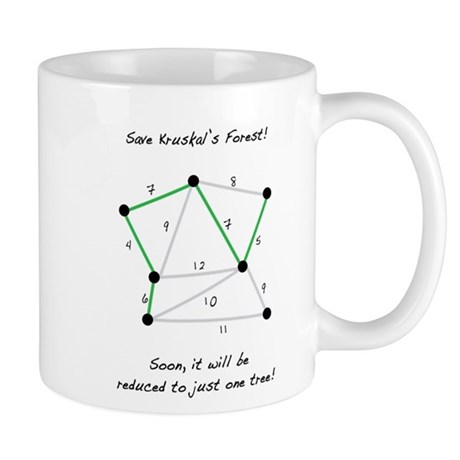
Put simply, a minimum spanning tree is a subset of the edges of a connected weighted graph that connects all the vertices in such a way that no cycles are created and the total edge weight is minimised. What’s with the forest then? Well, any weighted undirected graph has a minimum spanning forest, which is nothing more than the union of the minimum spanning trees for its connected components. That’s basically part of the joke on the mug. I know, it’s a homerun of a joke, and if you need to pause this read to catch a breath because of all your laughter, I would understand.

But now we know what a minimum spanning tree is, why care? What is it used for? Well, the applications are pretty numerous. The standard application is that of a telephone, electrical, TV cable or road grid. We want to connect all points with the least amount of cable/wire/road possible, since that’s a costly commodity. That’s basically the example I will elaborate a bit further on. However, several more out-of-the-box or indirect use cases do exist. You can use the algorithm to obtain an approximation of NP-problems such as the traveling salesman problem, for clustering data points in data science (although the K-means algorithm can also be used, depending on the application), in an autoconfig protocol for Ethernet bridging to avoid network cycles, and several others. To get the point across and explain the algorithm, we will use a classical road (or rather tunneling) problem.

Kruskal’s algorithm

So, finally, what you all came here for ;-) the algorithm itself. Kruskal’s algorithm uses a greedy approach (which means it follows the heuristic of making the optimal choice in each stage of the process) to solve the minimum spanning tree problem. It does so in a few, quite simple, steps:

1. Starting from a number of vertices, create a graph G where each vertex V is a separate tree. In short: no edges exist, just the trees.
2. Create a collection C containing all possible edges in G.
3. While C is non-empty and G is not yet spanning: remove the edge E with minimum weight from C. If E connects 2 different trees in G, add it to the forest, thereby combining 2 trees in a single new tree.

And that’s basically all there is to it. Additionally, you get the joke on the mug now. Starting from a forest of trees (non-connected vertices), you start connecting them using the possible vertices in increasing order, until there’s only 1 tree: the one containing all vertices, connecting those vertices with the cheapest possible edges that do not introduce cycles in the graph.

As I mentioned earlier - and as is often the case - the running time of the algorithm is dependent on the choice of your data structures. So let’s see what data structures I decided to use. Obviously we need a graph, which is the easy bit. I chose a straight forward adjacency list implementation. Also, we need a collection to store all edges in. We will perform repeated reads from that collection and pop out the cheapest remaining edge. I decided to use a priority queue in which the priority is the edge cost. I implemented this as a min binary heap. As a third and last data structure, I need something that allows me to recognise which trees belong together, as this enables me to detect cycles. When considering to connect 2 vertices by allowing the edge under consideration into the spanning tree, all I need to detect is whether they already belong to the same tree. A disjoint set is perfect for this. Let’s focus on each of the data structures first, after which we’ll look at the problem area, and the actual algorithm.

The graph

First and foremost, let me remind you that I’m doing all of this in Python. For our graph, we don’t really need anything fancy at all. All we need in this case is a simple dictionary with the vertices as keys, and a list with the neighbours of that key as value in order to save the graph as an adjacency list. I provided a number of simple dunder methods (the methods with the 2 underscores in front and back of them) for some basic operations we might want to execute on our graph, as well as a method to add a weighted edge to a vertex. For plain ease and simplicity, we just assume an undirected graph and delegate the burden of adding the edge back from neighbour to vertex to the graph. Vertices that don’t exist just get created on the spot. Again, just to keep things simple for the example. Check out the code below:

class Graph(object):
    def __init__(self, vertices=[]):
        self.__vertices = {vertex: [] for vertex in vertices}

    def __del__(self):
        self.__vertices = None

    def __len__(self):
        return len(self.__vertices)

    def __contains__(self, vertex):
        return vertex in self.__vertices

    def __getitem__(self, vertex):
        if not vertex in self.__vertices:
            return []
        return self.__vertices[vertex]

    def __iter__(self):
        for vertex in self.__vertices:
            yield vertex

    def add_edge(self, vertex, neighbour, cost):
        if vertex not in self.__vertices:
            self.__vertices[vertex] = []
        if neighbour not in self.__vertices:
            self.__vertices[neighbour] = []
        if (neighbour, cost) not in self.__vertices[vertex]:
            self.__vertices[vertex].append((neighbour, cost))
        if (vertex, cost) not in self.__vertices[neighbour]:
            self.__vertices[neighbour].append((vertex, cost))

The priority queue

As mentioned, our next main building block is the collection to store the edges in, as well as getting them out in ascending order of cost as cheaply as possible. This is pretty vital, as it greatly determines the running cost of the entire algorithm. That’s why I chose one of my favourite little data structures: the min binary heap to implement a priority queue. Again, it’s adjusted for this example, and I know it’s not Pythonic to leave out docstrings or use names like “i” or “j”, but bear with me here.

class MinBinaryHeap(object):
    def __init__(self, *values):
        self.__elements = [values]
        self.__check_elements = set(value for value in values)
        self.__ubound = len(values) - 1
        self.__build_heap()

    def __del__(self):
        self.__elements = None
        self.__check_elements = None

    def __contains__(self, element):
        return element in self.__check_elements

    def __str__(self):
        return ", ".join([str(el)
                    for el in self.__elements[0:(self.__ubound + 1)]])

    def empty(self):
        return self.__ubound == -1

    def push(self, value):
        self.__check_elements.add(value)
        self.__ubound += 1
        if self.__ubound > len(self.__elements) - 1:
            self.__elements.append(value)
        else:
            self.__elements[self.__ubound] = value

        self.__sift_up(self.__ubound)

    def peek(self):
        return self.__elements[0]

    def pop(self):
        if self.__ubound == -1:
            return None

        element = self.peek()
        self.__remove(0)
        return element

    def __build_heap(self):
        for i in range(int(self.__ubound / 2), -1, -1):
            self.__sift_down(i)

    def __sift_up(self, i):
        if i <= 0 or i > self.__ubound:
            return

        parent = int((i - 1) / 2)
        if self.__elements[parent][1] > self.__elements[i][1]:
            self.__swap(parent, i)

        self.__sift_up(parent)

    def __sift_down(self, i):
        if i < 0 or i > (self.__ubound - 1) / 2:
            return

        left = (i * 2) + 1
        if left > self.__ubound:
            return
        right = (i * 2) + 2

        if (right > self.__ubound or
            self.__elements[left][1] < self.__elements[right][1]):
            if self.__elements[i][1] > self.__elements[left][1]:
                self.__swap(i, left)
                self.__sift_down(left)
        else:
            if (right <= self.__ubound and
                self.__elements[right][1] < self.__elements[i][1]):
                self.__swap(i, right)
                self.__sift_down(right)

    def __remove(self, i):
        if i < 0 or i > self.__ubound:
            return

        element = self.__elements[i]
        self.__check_elements.remove(element)
        self.__swap(i, self.__ubound)
        self.__ubound -= 1
        self.__sift_down(i)

    def __swap(self, i, j):
        (self.__elements[i],
         self.__elements[j]) = (self.__elements[j],
                                self.__elements[i])

I will refrain from going too deep into the implementation of the data structure, because it would take me an entire article to do that alone. Please read up on binary heaps to learn more. What’s important to know right now is that all edges and their costs are stored in a simple list, that is then reordered in such a way that it adheres to a few core properties of a min binary heap:

• The shape property: the list translates to a complete binary tree (which is basically already the case since I store all values in a list and calculate the locations of all children in a naive way)
• The heap property: the value of each node in the tree is smaller than (or equal to) each of the nodes below it.

This does NOT mean that the list is ordered, by the way! That’s the main strength of the min binary heap and the heapsort algorithm it enables. We do not need to sort the entire list. All we need to do is reorder the list to satisfy those properties, which is why the build_heap method only operates on edges in the first half of the list. After all, the lowest half of the elements represent the leaves in the tree (remember, we double up the amount of nodes at each level of the binary tree), and the heap property is already satisfied for leaves. The 2 main components of the binary heap are the sift_up and sift_down operations, which basically make sure that a node is bubbled up or down the tree so that it’s in the correct position to satisfy the min binary heap properties. They maintain these properties during all the pushing and popping we do when working with the tree. The worst case runtimes of those 2 operations equal to O(log n) where n is the number of elements in the tree (which is basically the height of the tree).

All in all, since we have to get all edges out of the priority queue and consider them, the eventual running time for this part of the algorithm is O(n log n) with n being the number of edges, which is basically optimal for a comparison sort.

The disjoint set

The last component before getting into the algorithm itself is the way we determine which trees belong together in order to detect cycles, as well as merging trees. A great one for that is the disjoint set data structure, which is also known as the union-find data structure. That basically sums up what we are trying to do, right? Again, no great detailed explanation here, since that would take this article too far, but I’ll at least provide some information. Read up on it if you want to expand your knowledge on this.

class DisjointSet(object):
    def __init__(self, values):
        self.__parents = []
        self.__ranks = []
        self.__values_to_indices = {}
        for i, value in enumerate(values):
            self.__parents.append(i)
            self.__ranks.append(0)
            self.__values_to_indices[value] = i

    def __del__(self):
        self.__parents = None
        self.__ranks = None
        self.__values_to_indices = None

    def __get_parent(self, index):
        if index != self.__parents[index]:
            self.__parents[index] = 
                self.__get_parent(self.__parents[index])

        return self.__parents[index]

    def get_parent_index(self, element):
        return self.__get_parent(self.__values_to_indices[element])

    def merge(self, element1, element2):
        index1 = self.get_parent_index(element1)
        index2 = self.get_parent_index(element2)

        if index1 == index2:
            return
        
        if self.__ranks[index1] > self.__ranks[index2]:
            self.__parents[index2] = index1
        else:
            self.__parents[index1] = index2
            if self.__ranks[index1] == self.__ranks[index2]:
                self.__ranks[index2] = self.__ranks[index1] + 1

In short, we store our values in several ways. in values_to_indices (what’s in a name, right?) we basically have a dictionary that will tell us at which index in the parents and ranks lists each value is stored. Each entry in parents holds the index of the parent of the value at that index. I know that sounds like gibberish, so I’ll clarify with an example. Let’s say we have 4 values: “a”, “b”, “c”, “d”. Then our variables look like this:

self.__parents == [0, 1, 2, 3]
self.__ranks == [0, 0, 0, 0]
self.__values_to_indices == { "a": 0, "b": 1, "c": 2, "d": 3}

Which means that “a” points to index 0 in parents and ranks, “b” to index 1 and so on. In parents, we see that the element at index 1 has the element with index 1 as a parent. Same for 0, 2, 3. Basically, they all have themselves as parent, which means they just stand on their own. When merging 2 elements, we get their parent indices (using the path compression heuristic along the way - again, read up on it), and if they are different, it means they belong to different sets and can be merged. When doing the merging, we perform a union-by-rank (read, read, read) to keep our tree as shallow as possible in order to minimise running times. Let’s assume we want to merge elements “b” and “d”. The parent of “b” sits at index 1, the parent of “d” at index 3. So, they are not in the same set. We can then merge them, and we do so by setting the parent of “b” to be “d”. Since they both have the same ranks (0), element “d” sees it’s rank increased to 1. After that, our variables look like this:

self.__parents == [0, 3, 2, 3]
self.__ranks == [0, 0, 0, 1]
self.__values_to_indices == { "a": 0, "b": 1, "c": 2, "d": 3}

Elements “a” and “c” at index 0 and 2, respectively, still have themselves as parent, meaning they represent separate sets. Also, they kept their ranks as we didn’t touch them in this merge operation. However, element “b” at index 1 now has the element at index 3 as its parent. That would be “d”, as values_to_indices tells us. Element “d” itself didn’t change in terms of parent (meaning it’s still at the top of its tree), but did see its rank increase, since we took the rank of its new child “b”, increased it with 1 and assigned it to the rank of “d”. So we now have 3 sets: [“a”], [“c”] and [“d”,”b”]. That’s in simple terms how the disjoint set works. Thanks to the combination of the union-by-rank and path compression heuristics, our amortised running time per operation is lowered to O(α(n)), where α stands for the inverse Ackermann function. Details aside, this function has a result of <5 for any value of n that can be written in our physical universe. That makes disjoint set operations with these heuristics in place practically operate in constant time. That’s pretty awesome.

The algorithm itself

Now for the main event, the algorithm you all came to admire. For those expecting a great big codefest, spoiler alert: this will be a bummer. The code below is really all there is to it, thanks to good use of the data structures we created before.

def get_cost_minimal_spanning_tree(vertices, edgecoll):    
    # Kruskal's algorithm, just so you know, you might miss it
    total_cost = 0.0
    edges = MinBinaryHeap(edgecoll)
    minimal_tree = Graph(vertices)
    disjoint_set = DisjointSet(vertices)
    while not edges.empty():
        (vertex1, vertex2), cost = edges.pop()
        if(disjoint_set.get_parent_index(vertex1) != 
            disjoint_set.get_parent_index(vertex2)):
            disjoint_set.merge(vertex1, vertex2)
            minimal_tree.add_edge(vertex1, vertex2, cost)
            total_cost += cost
  
    return minimal_tree, total_cost

That’s messed up right? All of this reading for a few lines of code. But remember: all the heavy lifting is done by the data structures. They are what make or break this algorithm. That being said, we are in pretty good shape due to the choices we made. For this implementation, we assume we get the vertices and edges (with their costs) provided to us in lists vertices and edgecoll. The function not only creates the minimal spanning tree, but it also keeps track of the total cost of the tree so far, and returns them both as a tuple.

An example

Let’s demonstrate with a simple example where Joseph, Robert, Otto, Jarnik and Peter (inside joke) live in the same neighbourhood, and they want to create an underground tunnel system between their houses. I don’t know why, but there have been blockbusters making millions of dollars that had worse plots than this, so bear with me. Now, since they’re scientists, they don’t want to put too much work into this, as they have to research some new algorithms (hint to the joke) and want to maximise the time for that. So they want to connect all their houses with the least amount of tunnel needed to get the job done. I can’t give you any hint that is more obvious as to how to measure that. Minimum spanning trees to the rescue!

To simplify, we will use simple (x,y) coordinates to determine the locations of their houses. The coordinates for each house are:

• Joseph: (0, 0)
• Robert: (0, 2)
• Otto: (1, 1)
• Peter (3, 2)
• Jarnik (3, 0)

If we were to plot these locations on an imaginary chart, we would end up with something like this:

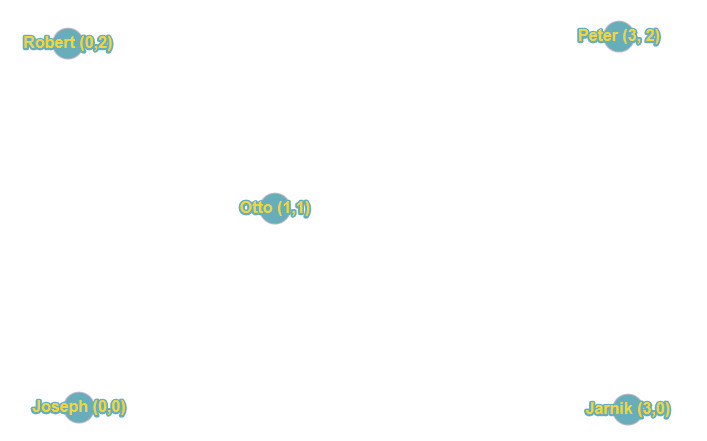
which makes for a decent enough estimation of the relative locations of the houses. Next up, we need to consider all possible tunnels (edges in the graph) we can dig between each of the houses. Simple graph theory tells us we will have (n * (n-1)) / 2 edges to check, where n is the number of nodes or houses. Thus, we will have 10 edges to go through, which cover all possible edges between all of the houses. As an example, this will suffice since we can easily reason about this, as well as visualise it. When considering this type of problem in real life however, when connecting hubs on a network or houses in a telephone grid or power grid, it’s easy to imagine the need for a fast algorithm, as the number of candidate edges will quickly run in the millions.

Besides building a list of all possible edges, we need to calculate the cost per edge. For our example, the costs are just Euclidean distances. I’m sure you remember your math from long ago, but as a reminder, we just take the Pythagorean theorem A² + B² = C² and give it a spin, giving us a simple way to calculate the distances in this 2-dimensional plane. By way of example, the distance between Otto and Peter is the root of ((3-1)² + (2-1)²), which equals to 2.24 (rounded up to 2 decimals). In this way, we calculate the costs between all nodes and add them to the edges, achieving the situation below:

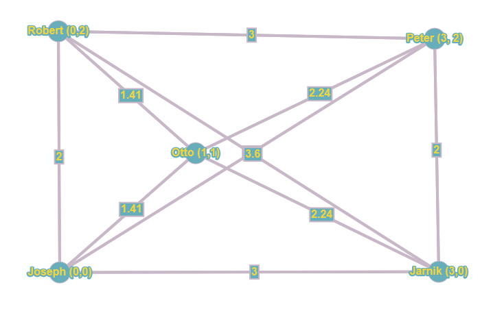
This is basically our starting point, our initial graph from which we need to distill our minimum spanning tree. I would invite you to once again read the algorithm steps, summarized for your convenience:

1. Create a graph G where each vertex V is a separate tree. We did that when plotting out all houses on our imaginary chart.
2. Create a collection C containing all possible edges in G. That’s the graph you found just above this list of steps. Our minimum spanning tree will consist of a subset of those edges, thereby connecting all points with the cheapest possible edges while avoiding cycles.
3. While C is non-empty and G is not yet spanning: remove the edge E with minimum weight from C. If E connects 2 different trees in G, remove it from the forest and add it to the spanning tree, thereby combining 2 trees in a single new tree.

And that’s what I leave up to you to work out for yourself. Again: we’re not in instant gratification land here ;-) it’s time to put those cells to work. But remember it’s quite simple: you will start from the graph without any edges. Then we start considering each edge in increasing order of cost. That would be either the edge between Robert and Otto, or Joseph and Otto. It doesn’t really matter. After that, the cheapest edge is that between Peter and Jarnik or between Robert and Joseph. Then the edges between Otto and Peter, and Otto and Jarnik are considered. When thinking about all those, watch out, since adding some could create a cycle, which you must avoid. Which ones you pick (in the case of equal cost) doesn’t really matter in the end result, your spanning tree could look slightly different, but the total cost remains the same). The next cheapest after that are the edges between Joseph and Jarnik, and between Robert and Peter. Again, watch out for cycles, and follow the steps in the algorithm and the logic in the data structures! Last edges are those between Robert and Jarnik and between Joseph and Peter. And that makes 10 edges you checked, depleting your priority queue, ending the algorithm and leaving you with the total_cost variable containing 7.06 as the minimum total cost, and a minimum spanning tree looking something like this:

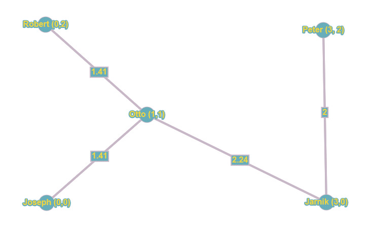
Again, the actual layout of your result could differ a bit, but the total cost should be the same. If the result you conjured up differs, you made an error in your reasoning somewhere, and I would encourage you to go over it again. So, to connect all their houses, the guys need to dig at least 7.06 (miles, meters, whatever your metric is) of tunnel. At least they found out fast enough, thanks to Joseph’s work. Now, some of the other guys also developed algorithms that are very similar, but I’ll leave that for you to discover ;-)

The running time

Now, how slow or fast is Kruskal’s algorithm? Well, as I said several times: it depends on the data structures. But to look at the running time, we should consider the 2 main steps:

1. Getting the sorted (by edge weight or cost) list of edges to consider: that’s where the binary heap comes in. It provides our edges in O(n log n) time, which is as good as it’s going to get for comparison sorting algorithms.
2. Processing each edge: thanks to the disjoint set, we can count on near-constant running times.

As we know, the total running time is determined by the slowest acting part of our algorithm. In this case, that’s the sorting of the edges. That makes Kruskal’s algorithm perform in O(|E| log |V|). Now, if there would be a scenario where some pre-processing was done, and the edges were already provided to us in increasing order, we would not need to perform the sorting work. This would imply we can achieve near linear running times, since we would perform a near-constant time operation for each edge, which would make the algorithm perform close to O(|E|) time.

And there you have it: my implementation and explanation of Kruskal’s algorithm. I hope you had a nice read and at least picked up some nice data structures to get you inspired. Feel free to copy the code and play around with it, keep in mind this is only really scratching the surface of all cool stuff out there, and remember that algorithms and data structures like these are the engines behind all the cool technology we have the privilege of using every day. So next time you consider a topic to study, give this a whirl. I promise you it will pay dividends in the future, and the JavaScript frameworks will still be there when you get back ;-)