Everybody and their grandma probably tried their hand at an implementation of Conway’s Game of Life at some point, in one or the other language. It’s a straightforward and elegant little algorithm that can give you cool looking results, and a nice goal to work towards while learning a language. Drilling plain syntax or frameworks is incredibly boring. When learning any new language, having a concrete goal in mind besides “just learning it”, helps speed the process along and makes it more enjoyable by far. So, while learning Python, I took a swing at it.
Game of what?
Just in case you haven’t Googled what I’m even talking about, the Game of Life is a cellular automaton designed by mathematician John Conway. It’s a game that requires just an initial input state, consisting of several alive and dead cells in a grid, after which the games’ rules take over and evolve the game from state to state:
- a live cell with less than 2 live neighbours dies by underpopulation
- a live cell with 2 or 3 live neighbours lives on
- a live cell with more than 3 live neighbours dies by overpopulation
- a dead cell with 3 live neighbours becomes a live cell
These few incredibly simple rules can manifest suprisingly complex patterns and really demonstrate the power of cellular automatons. The Game of Life is also Turning complete, and has been studied extensively. For more info, you can read up on it on Wikipedia, where you can take a much deeper dive into the subject.
My own spin on it
During this project, I familiarized myself with several language constructs and frameworks specific to Python, and tried several approaches to tackle the inherent slowness of Python for computational CPU-heavy work. You can check out a little summary video of what I’ll be working toward right here:
All the code is available on my GitLab. The complete code contains all the optimizations and little features I came up with.
One change I introduced, compared to the usual implementations you will find online, is that there are not 2 states for each cell, but 3:
- New: a cell that just became alive because of the game rules
- Survivor: an alive cell that hasn’t changed state in the current iteration
- Dead: a cell that is marked as dead, and will be removed from the game in the next iteration
This small change in how cells are visualized allows you to follow the evolution of each cell and the environment as a whole. Coupled with that, there are a number of inputs you can perform to interact with the grid:
- the game can be paused at any time
- a random cell layout can be generated
- several pre-built patterns can be added to the grid
- new cells can be injected into the grid
- alive and dead cells can switch places
- all surviving cells can be removed
- surviving cells that haven’t changed states in x iterations can be removed
- while the game is paused, you can move through the states one step at a time
- it’s possible to revert x amount of previous steps
- colors of all cells can be changed or reset to default values
- cell size can be changed to a predefined set of sizes
- target framerate can be changed
If you are interested in just a simple implementation with 2 states, you can checkout this branch. If you want to follow the evolution of the project from a basic implementation to using Numba to aid in faster computation of states, optimization of the search space, avoiding unnecessary recalculation of neighbours, and many other of the features above, there are a number of commits you can check out:
or just check out the develop branch for the finished product.
In the rest of the article, I will look at each of these commits and highlight what I consider the most interesting and fun things I worked on. I assume you have some basic knowledge of Python and virtual environments. The requirements.txt file to spin up your own is included, so you can simply check out the code, create your own environment and run the code. Throughout the different sections and checkouts, some stuff might be added to the requirements file, so be wary of the occasional necessity to install more packages ;-)
The basic implementation
So before we start getting creative, let’s get back to basics and look at what we will implement. In essence, all we need is a grid layout of cells, allow for some input by the user to mark cells as alive or dead, and a way to kick off the game. After that, it’s a matter of implementing the game rules iteratively, pushing each new state to the grid. Sounds simple enough. I used PyGame to implement the GUI. I’ve never been in love with front-end at all, but I was surprised by how easy PyGame was to get into and play around with. Besides PyGame, since we’re dealing with a grid of cells, the obvious choice is to go with NumPy to represent the data structure for the grid. Again, the code for this part can be found in this commit. Pretty much the only 2 functions that are worth talking about are the initialize and update functions:
def initialize(width: int, height: int, cell_size: int
               ) -> tuple[np.ndarray, pg.Surface, pg.time.Clock]:
    """Initialize all we need to start running the game"""
    pg.init()
    pg.display.set_caption("Game of Life")
    screen = pg.display.set_mode((width, height))
    screen.fill(GRID_COLOR)

    columns, rows = width // cell_size, height // cell_size
    cells = np.zeros((rows, columns), dtype=int)

    return cells, screen, pg.time.Clock()
It’s pretty clear what happens here. Besides setting up some boilerplate code to initialize PyGame, we create a simple matrix with zeros. A 0 at a certain position in the matrix represents a dead cell, whereas a 1 signifies an alive cell. This grid will then be taken as the input of the update function, in which we’ll calculate the new grid by applying the game rules to the current grid. We’ll also draw the rectangles that need to be redrawn based on the new situation:
def update(cells, cell_size, screen, running):
    """Update the screen"""
    updated_cells = np.zeros((cells.shape[0], cells.shape[1]), dtype=int)

    for row, col in np.ndindex(cells.shape):
        alive_neighbours = np.sum(cells[row-1:row+2, col-1:col+2]) - cells[row, col]
        color = BACKGROUND_COLOR if cells[row, col] == 0 else NEW_COLOR

        if cells[row, col] == 1:
            if alive_neighbours == 2 or alive_neighbours == 3:
                updated_cells[row, col] = 1
                if running:
                    color = SURVIVOR_COLOR
            else:
                if running:
                    color = DEAD_COLOR
        else:
            if alive_neighbours == 3:
                updated_cells[row, col] = 1
                if running:
                    color = NEW_COLOR

        pg.draw.rect(screen, color, (col * cell_size, row * cell_size,
                                     cell_size - 1, cell_size - 1))
    return updated_cells
An important line of code here is:
alive_neighbours = np.sum(cells[row-1:row+2, col-1:col+2]) - cells[row, col]
Here, we simply count the alive cells (the cells holding value 1) surrounding the cell under consideration. Since an alive cell has value 1, we can simply perform a summation. It also happens to be one of the most computational heavy lines of code in the whole algorithm. For each cell, we will count how many alive neighbours that cell has. It’s quite easy to see how this approach might become problematic as the gridsize increases, especially if we want to perform many updates per second and make the whole experience somewhat enjoyable to look at.
The result of the count will then determine the course of action for the considered cell. If it was alive (holding value 1), then we will color it as either a survivor (if it has 2 or 3 neighbours) or dead. For a dead cell, we will color it as a new cell if it has exactly 3 neighbours. This is simply the application of the game rules, with the aforementioned change that we will have 3 different cell states. Of course - for now - the states of the cell are only a visual feature since we color a brand new cell differently than a ‘survivor cell’. In the grid data structure, we do not make this distinction yet.
Besides these code snippets, you will not find much interesting in the basic implementation. There’s the main game loop, where the update function is called, and some event handling for marking and unmarking cells, and starting and stopping the game. When starting the game, all you need to do is click in the grid to mark a cell as alive. Rightclicking said cell marks it as dead. Hitting spacebar starts and pauses the game. So it’s simple to make a few clusters of cells (do yourself a favor and don’t click individual cells, you can just click-and-drag over cells to mark them alive or dead), and hit space to make the game start.
Let’s speed things up
When you run the game yourself, you will notice how small the PyGame window is:
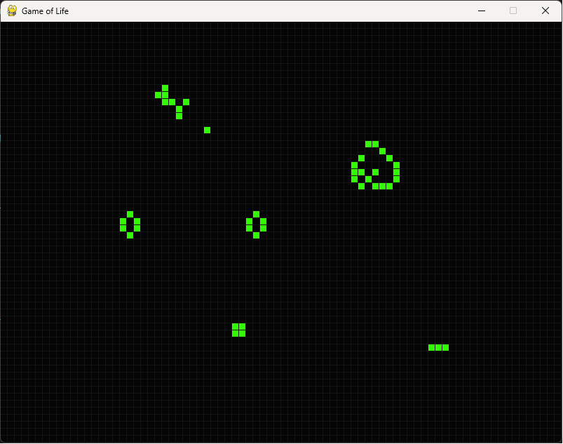 We have a very small window of 800x600 pixels, with a gridsize of 10 pixels. In short, our grid has 80 columns and 60 rows, for a total of 4800 cells. Even for such a small window, keep that one line of code in mind, where we count the number of neighbours of a cell… For each of those 4800 cells, we’ll have to perform a sum of the values of the 8 surrounding ones. Doesn’t seem too bright of an idea to start doing that several times a second (at least 60 times, since 60 frames per second does sound like an enjoyable experience), on a grid bigger than a little thumbnail.
So in the next section, we’ll make some big changes from our crude implementation into something that’s actually worth writing a blog about ;-) In case you do want to look at this step, check out this commit.
A dedicated grid class
Firstly, let’s create a class to express the grid, and hold all the game logic and ruleset. That way, the UI-related code is separated from the actual interesting stuff. So, from now on, all code in gameoflife.py will not be looked at anymore. Fiddle and inspect it if you feel like it, but you will find nothing particularly interesting in there. All it is, is setting up PyGame, responding to user inputs, updating the screen and handling the main game loop. The code that’s of actual interest all sits in conwaygolgrid.py. Most of the code in the class is fairly straightforward. The most important and interesting stuff happens in the update method, which changed pretty drastically from the previous iteration. In fact, the update function is now simply a pass-through to the static method __perform_update, in which the actual work is done.
    @staticmethod
    @njit(fastmath=True, cache=True)
    def __perform_update(cells: np.ndarray, background_color: tuple[int, int, int],
                         new_color: tuple[int, int, int],
                         survivor_color: tuple[int, int, int],
                         dead_color: tuple[int, int, int]
                         ) -> tuple[np.ndarray, list[tuple[int, int,
                                                     tuple[int, int, int]]]]:
        """Updates the grid to the next step in the iteration, following
        Conway's Game of Life rules. Evaluates each cell, and returns the
        list of cells to be redrawn and their colors
        """
        cells_to_redraw: list[tuple[int, int, tuple[int, int, int]]] = []
        updated_cells = np.array([[0] * cells.shape[1]] * cells.shape[0])
        for row, col in np.ndindex(cells.shape):
            alive_neighbours = (np.sum(cells[max(0, row-1):row+2,
                                max(0, col-1):col+2]) - cells[row, col])
            if cells[row, col] == 1:
                if alive_neighbours == 2 or alive_neighbours == 3:
                    updated_cells[row, col] = 1
                    cells_to_redraw.append((row, col, survivor_color))
                else:
                    cells_to_redraw.append((row, col, dead_color))
            else:
                if alive_neighbours == 3:
                    updated_cells[row, col] = 1
                    cells_to_redraw.append((row, col, new_color))
                else:
                    cells_to_redraw.append((row, col, background_color))

        return updated_cells, cells_to_redraw
You will also notice the decorator called njit. Besides that, the function now returns a tuple of the updated cells and the cells to redraw on the screen. So what is that all about? Simply: to remedy the fact that doing a lot of computation (however simple it is) in Python is always going to be slow, we use Numba. In a nutshell, Numba is a jit-compiler for Python which allows you to compile a decorated function to machine-code and execute it much faster. Numba works best on Numpy types, as well as basic for loops in Python. However, not all datatypes in Python are usable in Numba, and since the Numba-compiled code kinda runs separately, you can not simply pass in parameters and get them back as if you are writing plain Python. That is why the __perform_update function is marked as a static method, and data that is known in the class is still explicitely passed in instead of refering it using self.
Thanks to Numba, all the repetitive computation and looping that would be excruciatingly slow to have to suffer through in plain vanilla Python, will now be handled just fine. The arguments that are added to the njit decorator are further optimizations that will help the performance along. In short, fastmath relaxes numerical rigour (since we are simply performing a sum of 8 values in the neighbour cells and are not calculating highly accurate decimal numbers), and setting cache to True will cache the compiled code for next executions. The very first time an njit-decorated function is called, it needs to be compiled, so this first iteration is handled slightly slower. All other calls will call the cached compiled function and will execute very fast.
If you care to convince yourself of the difference between using Numba and not using it: comment out the
@njit(fastmath=True, cache=True)
line of code. The program will run just fine. However, you will notice that for any decent amount of drawn cells before you hit space to kick off the game, the speed will be dramatic. Performing a lot of CPU-heavy work in a loop is simply not what Python was made for. For your suffering/amusement, I added an fps counter in the bottom left. You’ll notice that I kicked up the screen size to 1920x1200 pixels, giving us a grid of 192 columns and 120 rows, which translates to 23040 cells to recalculate every iteration. In pure Python, that results in a less-than-enjoyable 3fps. Do yourself a favor and uncomment that decorator. It will result in about 20-30 fps. Still not quite great, but at least there’s some movement to behold without wondering if there’s something wrong with your computer.
I’d even say, if your idea of “fun” and “cool” is to watch a cellular automaton evolve semi-quickly, you should start developing warm fuzzy feelings right about now. If so, we’re on the same frequency. For the 4 guys reading this that are still following along, and to which that applies: keep reading, cause we can do better…
Let’s do even less
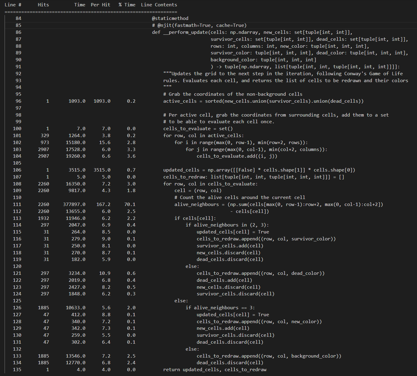
As often is the case when speeding up algorithms, we can achieve that by doing less. Sure, it’s nice to see an existing framework do some work for us and speed things up. But let’s pretend it’s not 2023, and we can’t depend on others to do the work for us. Let’s actually think for a second, and see what we’re doing. We’ll also use the help of line-profiler, which we can use to see the running time of certain functions. I don’t want to dive in too much details about this Python package here, but you can find more information about it here. In short, we will use it to diagnose the more costly operations inside of the __perform_update function. Since this is the main function of the game loop, it would be good to run this as fast as possible to be able maximize the number of game state calculations per second, and thus a more fluid experience. Running the profiling.py file in the current state will yield an output as follows:
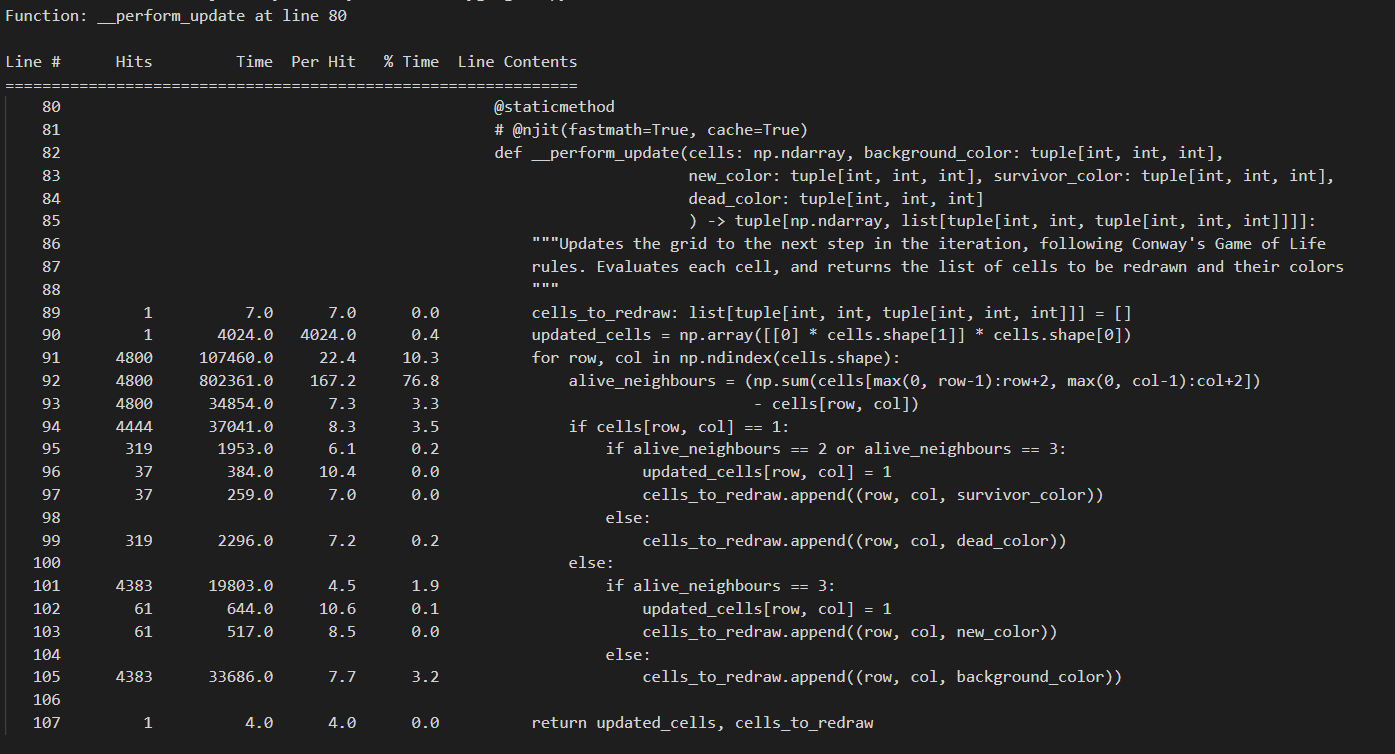 If you want to run this yourself, do make sure to comment out the njit-decorator first. line-profiler will only profile Python code. If you leave the njit-decorator active, the __perform_update function will be compiled into C-code, after which this compiled version will be called on, and we will not get any valueable data back from line-profiler. The profiling.py file just runs one iteration of the function using a 800x600 grid with cellsize 10, filled up with a random amount of alive and dead cells (well, there’s more chance for cells to be alive than dead to at least have a decent chunk of data to calculate). Looking at the results, we can immediately draw 2 conclusions:
- The calculation to determine the alive neighbours of a cell (which basically steers our entire ruleset) is performed 4800 times. In short: for every cell.
- Each individual calculation takes up a bit too much time. We slice up the Numpy array to get a subset of the cells, and then perform a sum on their values (0 or 1) to find out how many neighbours it has.
Some thoughts about these things: if we envision the complete grid, it’s not hard to imagine that most of the cells in the grid are dead and/or surrounded by dead cells. For those cells, no calculation would need to happen at all, as they would not have to change state from one iteration to the next. Additionally, as we traverse the grid from row to row, and column to column, we are bound to do double work. The neighbours of the cell at coordinates [0, 1] are at least partially the same as the neighbours of the cell at coordinates [0, 0]. However, we still slice up the array around each of those coordinates and pretend the work from the past (being the previous cell) never happened. That’s definitely a waste of time.
In short, performing memoization and shrinking the search space are 2 classical approaches we can apply to this problem to makes sure we are limiting the amount of work we do per iteration, and that the work we actually do is not lost. There are several approaches here, and it can sometimes become a balancing act between results and readability and complexity of the resulting code. Let’s go over the route I decided to take, and focus on the most important parts. You can find the actual code in this commit.
New representation of cells
We’ll focus on the new __perform_update function:
    @staticmethod
    @njit(fastmath=True, cache=True)
    def __perform_update(cells: np.ndarray, new_cells: set[tuple[int, int]],
                         survivor_cells: set[tuple[int, int]], dead_cells: set[tuple[int, int]],
                         rows: int, columns: int, new_color: tuple[int, int, int],
                         survivor_color: tuple[int, int, int],
                         dead_color: tuple[int, int, int],
                         background_color: tuple[int, int, int]
                         ) -> tuple[np.ndarray, list[tuple[int, int,
                                                     tuple[int, int, int]]]]:
        """Updates the grid to the next step in the iteration, following
        Conway's Game of Life rules. Evaluates each cell, and returns the
        list of cells to be redrawn and their colors
        """
        # Grab the coordinates of the non-background cells
        active_cells = sorted(new_cells.union(survivor_cells).union(dead_cells))

        # Per active cell, grab the coordinates from surrounding cells, add them to a set
        # to be able to evaluate each cell once.
        cells_to_evaluate = set()
        for row, col in active_cells:
            for i in range(max(0, row-1), min(row+2, rows)):
                for j in range(max(0, col-1), min(col+2, columns)):
                    cells_to_evaluate.add((i, j))

        updated_cells = np.array([[False] * cells.shape[1]] * cells.shape[0])
        cells_to_redraw: list[tuple[int, int, tuple[int, int, int]]] = []
        for row, col in cells_to_evaluate:
            cell = (row, col)
            # Count the alive cells around the current cell
            alive_neighbours = (np.sum(cells[max(0, row-1):row+2,
                                max(0, col-1):col+2]) - cells[cell])
            if cells[cell]:
                if alive_neighbours in (2, 3):
                    updated_cells[cell] = True
                    cells_to_redraw.append((row, col, survivor_color))
                    survivor_cells.add(cell)
                    new_cells.discard(cell)
                    dead_cells.discard(cell)
                else:
                    cells_to_redraw.append((row, col, dead_color))
                    dead_cells.add(cell)
                    new_cells.discard(cell)
                    survivor_cells.discard(cell)
            else:
                if alive_neighbours == 3:
                    updated_cells[cell] = True
                    cells_to_redraw.append((row, col, new_color))
                    new_cells.add(cell)
                    survivor_cells.discard(cell)
                    dead_cells.discard(cell)
                else:
                    cells_to_redraw.append((row, col, background_color))
                    dead_cells.discard(cell)
        return updated_cells, cells_to_redraw
Quite the change, quite some more incoming arguments, but as you will hopefully realize, the complexity didn’t grow that much whereas the increase in speed did. To reiterate, our previous implementation had 2 issues:
- We perform a calculation for each cell in the grid. This doesn’t scale when the grid becomes large.
- Each calculation ignores the previous work being done (being the neighbour count for cells that have overlapping neighbours)
To remedy this, I have introduced a few simple changes:
- Instead of holding the grid in a simple Numpy matrix, I also introduced dedicated sets for alive, survivor and dead cells. Each of these sets only hold the coordinates of the cells in that respective state. At any point in time, we know which cells are in which state.
- The result of that change (which basically is an increased space complexity to achieve a better time complexity) enables us to just take the coordinates of cells that are either new from the previous iterations, surviving from the previous generation, or newly marked as dead because of the application of the game rules in the previous iteration. Any cell that is just “part of the background” and which wasn’t even changed in the previous iteration, is not even taken into consideration for calculation of the next game state. As a reminder: for most of the runtime of the game, that’s actually most of the cells in the grid. In short, just like that, we could cut out most of the work in each loop.
An important detail here of course, is that it’s not ONLY the active cells (new cells + survivor cells + dead cells) that will be potentially changing state in the next iteration of the game, but also their immediate surrounding cells. In short, once we know the coordinates of all active cells, we add them and their immediate surrounding cells to a set, which will result in a collection of cells that we will have to calculate the next game state for. We use a set so we have an easy built-in way to avoid adding the same cell twice.
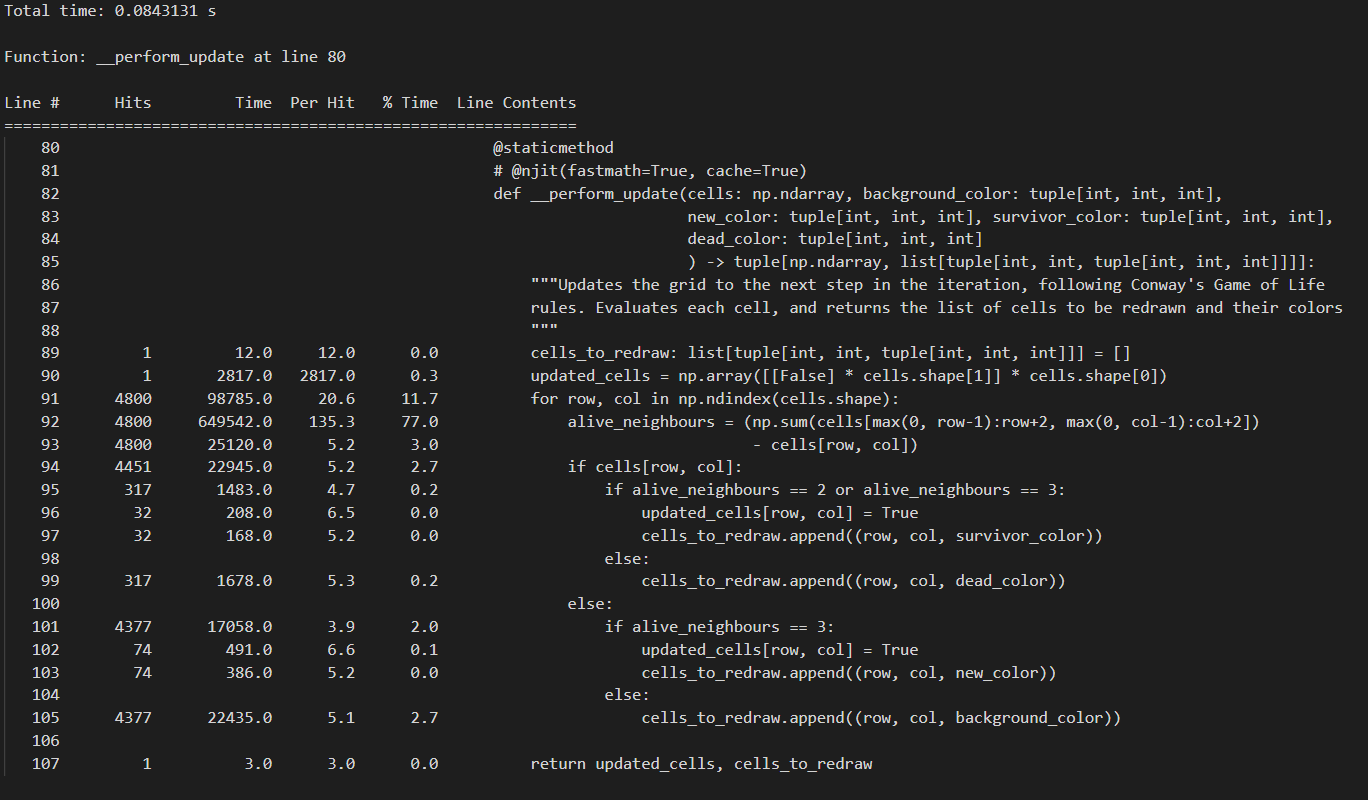
In essence, we still do the same thing in the new function: we iterate over the cells we want to take into consideration, count the alive neighbours of that cell and simply apply the basic game rules to that cell. We need to of course apply some extra bookkeeping to make sure each of our sets hold the correct cells at any point in time, but this is trivial. If we run the profiling on these changes, an example output looks as follows:
 Some conclusions here:
- Grabbing the active cells by taking the union of the individual sets for new, surviving and dead cells is cheap. Also, it’s just performed once.
- Taking the surrounding cells of these active cells, yielding us the list of cells we want to perform the main calculations on, is also a lightweight operation.
- Counting the neighbours per cell is still a costly operation, we didn’t really change this, but: we perform this MUCH less. As opposed to doing this for each cell, in each iteration (which would be 4800 times for a 800x600 grid of cellsize 10), we only do this 2260 times in this case. And remind yourself: this is for a grid that is very filled up, which will be quite rare, and close to a worse case scenario.
Besides just looking at numbers, start the application (don’t forget the uncomment the njit-decorator if you commented it to generate the profiling results). Notice I kept the screen size of 1920x1200 the same, but have change the cell size to 5x5 pixels. That means 384 columns and 240 rows, and as such, 92160 cells to handle. And still, instead of reaching 20-30fps, we are now reaching 30-40fps for more than 3 times the amount of cells! In fact, to be snarky about it, comment out that njit-decorator again. You’ll reach about 10fps. That’s not great in itself, but think back to the first implementation. We had a 800x600 grid with 4800 cells, and reached 3fps using pure Python. Now, due to the optimization we built in ourselves instead of relying on precompiled highly-optimized code, we reach 10fps in a grid with 92160 cells. Sometimes, even if it’s just as an exercise for yourself, it’s just more satisfying to think outside the box instead of relying on pre-built tools to do the job for you. And the combination of both can yield great results.
Now, this is by no means an upper limit of what you can reach. However, it’s a fun optimization to reach, despite having to deal with a language that is really not built or suited for this kind of work. Build this project in C++ or Rust if you want to see real speed. For Python though, I’d call this a satisfying result. Remember: we are still calculating the neighbours of each cell individually. You COULD perform some memoization there and re-use the work you performed for previous cells. There are many ways to do this, again with varying added complexity as a result.
A different way to count neighbours
Let’s inspect how I decided to do it, and checkout this commit. The new __perform_update function looks like this:
    @staticmethod
    @njit(fastmath=True, cache=True)
    def __perform_update(cells: np.ndarray, neighbour_count: np.ndarray,
                         new_cells: set[tuple[int, int]],
                         survivor_cells: set[tuple[int, int]],
                         dead_cells: set[tuple[int, int]],
                         rows: int, columns: int,
                         new_color: tuple[int, int, int],
                         survivor_color: tuple[int, int, int],
                         dead_color: tuple[int, int, int],
                         background_color: tuple[int, int, int]
                         ) -> tuple[np.ndarray, list[tuple[int, int,
                                    tuple[int, int, int]]]]:
        """Updates the grid to the next step in the iteration, following Conway's
        Game of Life rules. Evaluates each cell, and returns the list of cells
        to be redrawn and their colors
        """
        # Grab the coordinates of the non-background cells
        active_cells = sorted(new_cells.union(survivor_cells).union(dead_cells))

        # Per active cell, grab the coordinates from surrounding cells,
        # add them to a set to be able to evaluate each cell once.
        cells_to_evaluate = set()
        for row, col in active_cells:
            for i in range(max(0, row-1), min(row+2, rows)):
                for j in range(max(0, col-1), min(col+2, columns)):
                    cells_to_evaluate.add((i, j))

        updated_cells = np.array([[False] * cells.shape[1]] * cells.shape[0])
        neighbour_count_to_update: list[tuple[tuple[int, int], int]] = []
        cells_to_redraw: list[tuple[int, int, tuple[int, int, int]]] = []
        for row, col in cells_to_evaluate:
            cell = (row, col)
            # Count the alive cells around the current cell
            alive_neighbours = neighbour_count[row, col]
            if cells[cell]:
                if alive_neighbours in (2, 3):
                    updated_cells[cell] = True
                    cells_to_redraw.append((row, col, survivor_color))
                    survivor_cells.add(cell)
                    new_cells.discard(cell)
                    dead_cells.discard(cell)
                else:
                    cells_to_redraw.append((row, col, dead_color))
                    neighbour_count_to_update.append((cell, -1))
                    dead_cells.add(cell)
                    new_cells.discard(cell)
                    survivor_cells.discard(cell)
            else:
                if alive_neighbours == 3:
                    updated_cells[cell] = True
                    cells_to_redraw.append((row, col, new_color))
                    neighbour_count_to_update.append((cell, 1))
                    new_cells.add(cell)
                    survivor_cells.discard(cell)
                    dead_cells.discard(cell)
                else:
                    cells_to_redraw.append((row, col, background_color))
                    dead_cells.discard(cell)

        for coordinates, delta in neighbour_count_to_update:
            row, col = coordinates
            for i in range(max(0, row-1), min(row+2, rows)):
                for j in range(max(0, col-1), min(col+2, columns)):
                    if (i, j) != coordinates:
                        neighbour_count[(i, j)] += delta

        return updated_cells, cells_to_redraw
You will notice it’s pretty much the same as in the last commit, except for one crucial change:
alive_neighbours = neighbour_count[row, col]
and later in the function:
for coordinates, delta in neighbour_count_to_update:
    row, col = coordinates
    for i in range(max(0, row-1), min(row+2, rows)):
        for j in range(max(0, col-1), min(col+2, columns)):
            if (i, j) != coordinates:
                neighbour_count[(i, j)] += delta
In short, we have introduced a new matrix of the same size as the grid. Each cell will simply hold the amount of neighbours of the cell at that index. When initializing the grid, obviously each value holds a zero. Then, as the user clicks a cell, or as we calculate the new state of each cell, we perform updates to that matrix. This approach to optimizing the “counting of neighbours” problem is called amortization. You can read about it here, but simply put, it is an approach to defer the cost of a (time-wise) expensive operation and simply spread it out over time instead of having to suffer the full brunt of it all at once. This is one of many ways to do memoization in algorithms.
Very simply put: instead of calculating all neighbours for each cell in each iteration, we remember the amount of alive neighbours for each cell, and update that value whenever it changes. This guarantees that whenever we want to know about the neighbours of each cell at the start and we can just fetch that value in constant-time. This trade-off of performing a bit of extra working when we change the state of a cell, as opposed to counting the neighbours for each cell even though that cell didn’t even change state, will result in even faster game state calculation.
If you run the program, you will notice that (unless you completely overload the grid with alive cells) it will reach 50-60fps now. And even while commenting out the njit-decorator, reverting us to pure Python and not having the luxury of a precompiled optimized C-function, we get close to 20fps.
Some more numbers…
Besides actually looking at the game play out, and seeing the obvious speed changes from commit to commit, let’s check out a commit with no code changes, but where I have added 3 profiling results:
- profiling_results_numba_only: the optimized results due to the use of Numba only
- profiling_results_smaller_searchspace: as the previous, but we limited the searching space as explained earlier
- profiling_results_optimized_neighbour_count: more of the same, but we also changed the way we count neighbours
In fact, if you are still reading this, you MUST be a developer, and hence you are lazy. Instead of checking out the code, here are the screenshots of these profiling results:
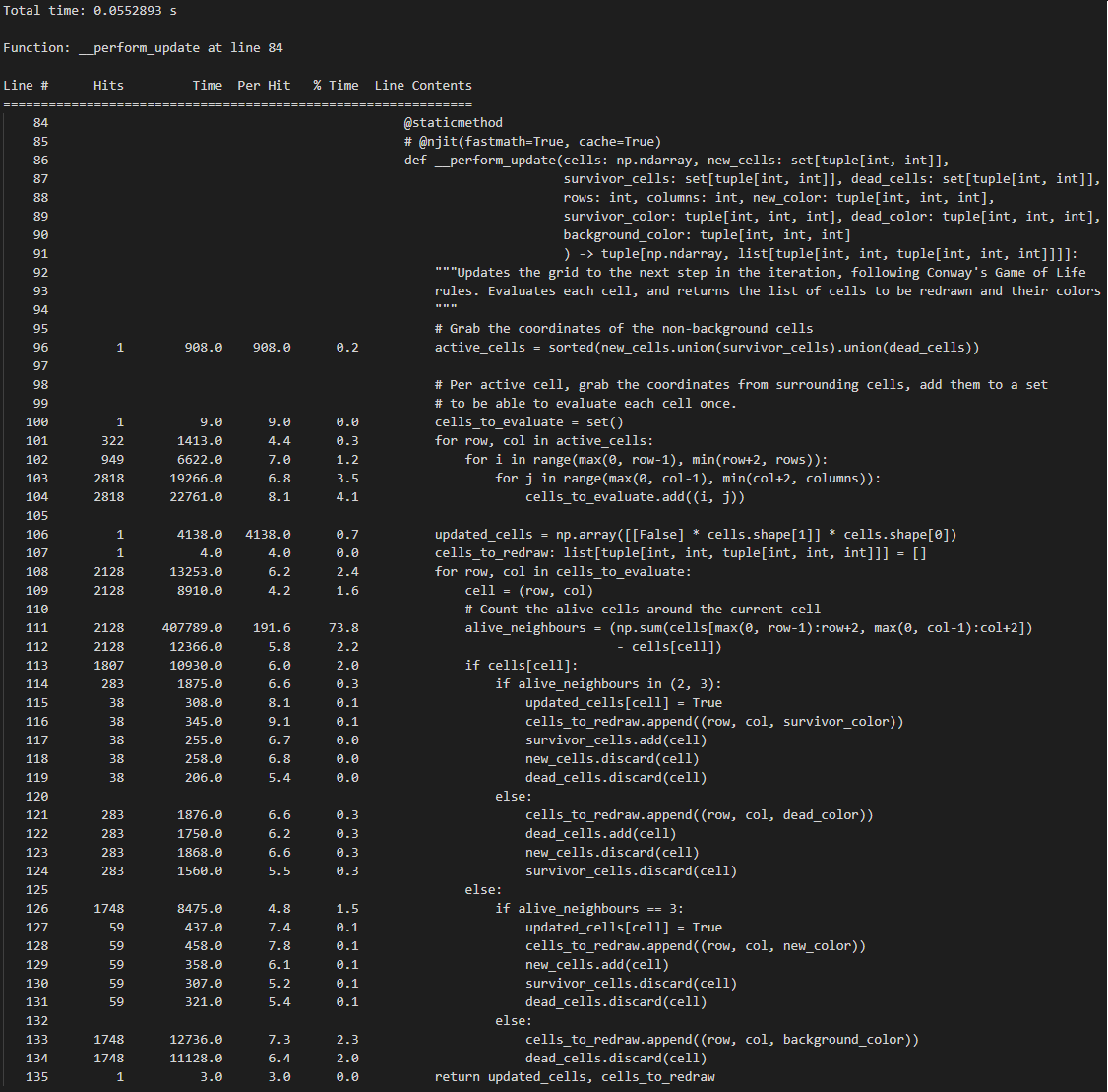
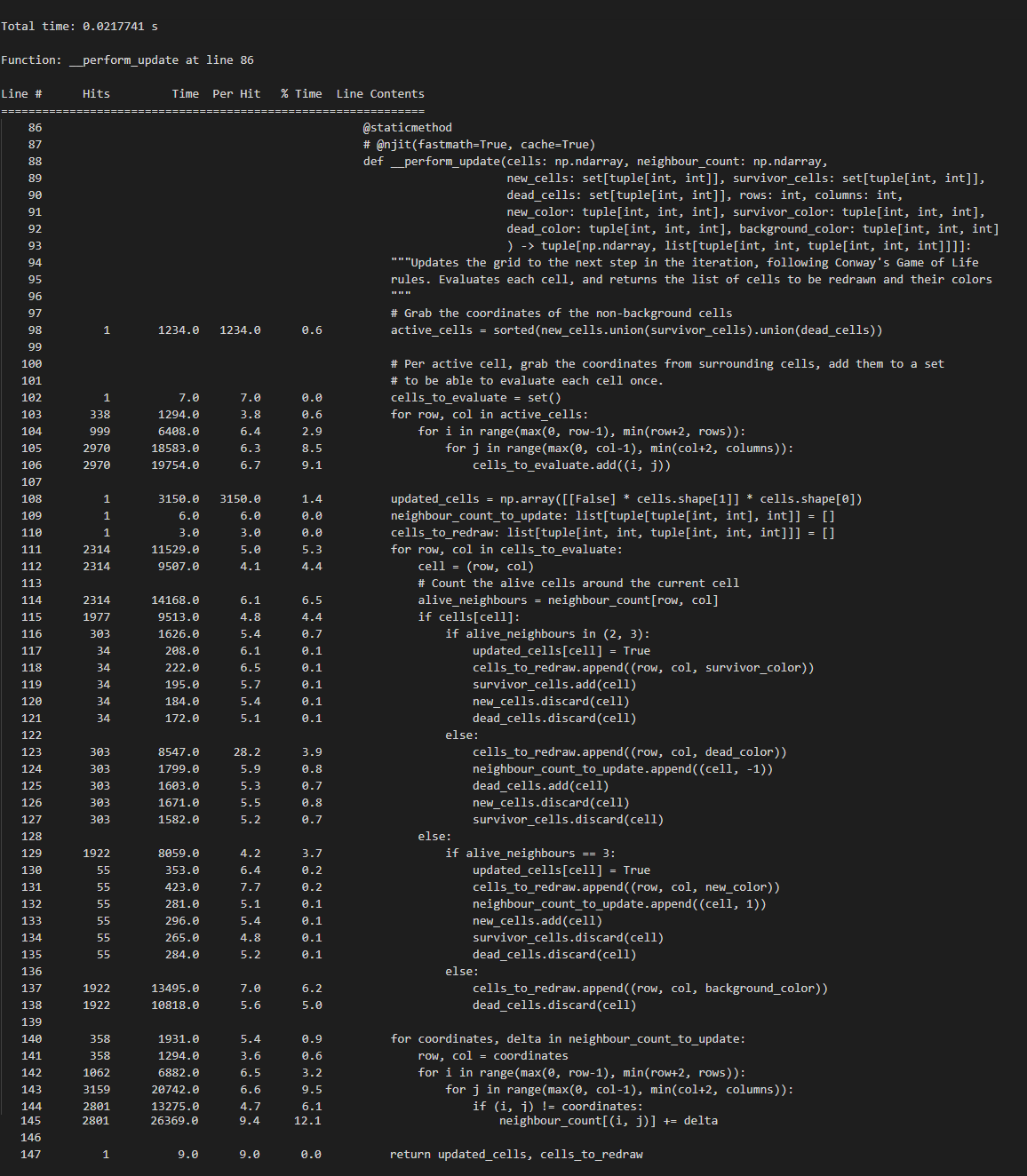
Now, this is just a sample of course, but a single calculation of a new game state on a 800x600 grid with cellsize 10x10 pixels went from 0.084secs with Numba to 0.055secs by limiting the searchspace, to 0.021secs by optimization of the neighbour count. So, although Numba definitely unlocked a big speed gain, some cricital thinking concerning the actual work, and a few simple changes, granted us a 4x speed increase, even though we used a language that is not really built for a lot of computation.
In reality, we kind of danced around that problem by moving the complexity from time to space, and just did less computation. It’s not hard to imagine that if we use a compiled language that’s more suited to this kind of work like C++ or Rust, we’ll reach much better performance. Turning that argument on its’ head though: if we did use those languages to solve this, we wouldn’t have even considered our optimizations because the language would have done most of the work for us.
Using Python for this type of little project does unlock a lot of ways to have fun. You can use frameworks that do a lot of work for you, like Numpy and Numba, but if you care to dig deeper, the sheer fun of the language and the easy syntax of it encourage you to try out new approaches. Before I converged on the current implementation, I really tried many different approaches for counting neighbours and such. Because of how easy it is to write Python, you can iterate on solutions and prototype very quickly. And ironically, simply because it wasn’t made for computationally heavy work, you can mimic the 80’s and 90’s again, where you had to depend on your own enginuity and creativity to use the tools and knowledge under your belt to come up with a good solution under certain hardware (or in this case, language) constraints.
In fact, this frame of mind made me get into solving the traveling salesman problem using Python in 4 different ways. That’s for my next blog though, although you can already see the results right here. I had a lot of fun with that one, especially the genetic algorithm and ant colony optimization implementations. Something I always wanted to try, but finally got around to.
Features…
However… before getting to that: after I implemented the optimizations I mentioned above, and saw that I could reach quite a decent framerate, I decided it was time to stop thinking too much and just have some fun with it. If you check out the last version of the develop branch, you’ll find that the code changed quite a bit. Just start the program and press F1 when you see the PyGame window appear, and you will get a short summary of what you are able to do. Again, the results of that are summarized in this YouTube video, but I leave it to you to play around with it, and maybe use it as an inspiration to optimize it even further and just run with it. I think especially the manual step forward and revert functionality can be handy to learn about the way the Game of Life works, if that’s your cup of tea. If that’s not your deal and you just want to experiment with self-induced epilepsy, have at it and change colors in an overly crowded grid. Don’t say I made you. Just a hint: throwing on a few of the eternal generator presets I built in, as well as overlaying the grid with the cross-pattern repeatedly as it runs, can yield pretty cool results and long-running games. Again, my idea of fun might slighty diverge from yours.
Thank you for reading this entire blog, I’m sure there’s more enjoyable and relaxing ways to spend your time on the internet. There is still a very large amount of things I could talk about concerning the implementation of several features, the profiling, the caching of cells bloomed with OpenCV,… If you have any questions, remarks or interesting thoughts to share, let me know! If you improve on the implementation or have ideas on how to possibly optimize it further, don’t hold back on either implementing it yourself and sharing the results, or plant that seed in my mind by sharing. I might just be crazy enough to start doing it. Again, thanks for reading this blog, you did it to yourself, but I thank you all the same ;-)