
The traveling salesman problem is one of those annoying interview questions you sometimes get hurled at you, accompanied by “How would you solve this”? I remember a time when I was a fresh hatchling straight out of college, finding myself in that exact situation. I’ll spare you the details, but I can tell you I didn’t get particularly far 😉
Times change, though, and over the years I grew into the type of software engineer that definitely prefers to work with data structures and algorithms over the next “best” framework used to make text and images appear in a web browser. If that happens to be your cup of tea, don’t get too offended; I’m an UI-ignorant back-end kind of guy, and you will undoubtedly run circles around me if it comes to any front-end related tech.

Some solutions…
Now, quite a few years later, I thought it’d be a nice moment to provide a few potential solutions, and give you a little bit of a summary regarding how to go about it. I assume you know what the Traveling Salesman Problem entails, at least from a high level. In short, the goal is to find the Hamiltonian cycle in an undirected weighted graph with the lowest cost. It’s one of those nice annoying NP-hard problems, so more than enough ways to have fun with it. It has many applications, from planning, logistics to manufacturing microchips. In this article, I’ll go over 4 example implementations of possible solutions to the problem:
- a simple brute force algorithm, guaranteed to give you the optimal shortest distance, but obviously horribly slow
- another guaranteed optimal solution, but quite a bit more efficient, using dynamic programming
- an approximation of a solution using genetic algorithms
- another approximation, using ant colony optimization
I’ve been interested in genetic algorithms and ant colony optimization for a while now, and the traveling salesman problem is a nice use-case to apply these algorithms to. In case you are not familiar with one or both of them, you can find more information about Genetic algorithms and Ant Colony Optimization all over the internet. Or you can ask ChatGPT, apparently that’s quite the trend lately. There are several other ways to go about finding solutions, like simulated annealing, n-opt and several of its variations, but I wanted to stick to what triggered my curiosity the most.
The project
The full code of the project is available on my GitLab. The requirements to run it are pretty basic. It’s all Python code, and I mainly use PyGame, Numpy, Asyncio and Aiostream. Just install the requirements in requirements.txt and you’ll be set. You can preview the end result right here:
In fact, give that a quick gander, keep it open in your browser to get back to every now and then, and the rest of the article will quickly become clear. Obviously, cloning it yourself and running it will help your understanding even more.
The PyGame window that pops up when running shows you 5 panes. The top center one is the one where you can left-click to add points. These points will be the destinations our supposed salesman will have to visit. The first point you create will be green, and will be the starting point and end destination. All other blue ones are the cities to be visited before getting back to the starting point. Hitting the spacebar will reset the screen, enter starts the algorithm. The distances between points are simply the Euclidean distance in pixels between the points.
Since brute force and dynamic programming solutions are inherently slow for anything more than a few points, you’ll notice there’s a cut-off point where those algorithms are not being taken along for the ride anymore. It would simply take too much time, as the time complexity for both just explodes when the amount of points gets too high. Dynamic programming will be used for a bit longer than brute force, but when you start getting in the double digits in terms of destination count, both will not be executed anymore.
In case you do follow along in the code and check out the GitLab project, there aren’t a lot of files of interest:
- main.py: nothing you wouldn’t expect. The only code of slight interest there is how to run the 4 algorithms concurrently. All the rest is setup for PyGame, running the main “game loop”
- graph.py: contains an implementation of an undirected weighted graph, slightly tailored to the current problem at hand
- the folder /solvers contains the implementations of the 4 algorithms. The rest of the article will mostly focus on those
Processing the results
As stated earlier, the main.py file doesn’t contain much regarding the actual problem. However, maybe one little thing to touch on is how the 4 algorithms are executed concurrently, and results are processed as they come in.
algorithms = [algorithm for algorithm in self.__algorithms
              if algorithm is not None]
zipped = stream.ziplatest(*algorithms)
merged = stream.map(zipped, lambda x: dict(enumerate(x)))
async with merged.stream() as streamer:
    async for resultset in streamer:
To explain what goes on there, we’ll consider the following simple example:
import asyncio
from aiostream import stream


async def process_results_interleaved(races):
    combine = stream.merge(*races)
    async with combine.stream() as streamer:
        async for item in streamer:
            print(item)


async def process_results_packet(races):
    zipped = stream.ziplatest(*races)
    merged = stream.map(zipped, lambda x: dict(enumerate(x)))
    async with merged.stream() as streamer:
        async for resultset in streamer:
            print(resultset)


async def race(racer, sleep_time, checkpoints):
    for i in range(1, checkpoints + 1):
        await asyncio.sleep(sleep_time)
        if i == checkpoints:
            yield f"{racer} finished!"
        else:
            yield f"{racer} hits checkpoint: {i}"


def create_races(checkpoints):
    return [race("Turtle", 2, checkpoints),
            race("Hare", 1, checkpoints),
            race("Dragster", 0.3, checkpoints)]


def main():
    checkpoints = 10

    print("Starting race, processing results as they come in from each contestant:")
    races = create_races(checkpoints)
    asyncio.run(process_results_interleaved(races))

    print("Starting race, processing results in packets:")
    races = create_races(checkpoints)
    asyncio.run(process_results_packet(races))


if __name__ == "__main__":
    main()
Just go over the code real quick, and it’ll become pretty clear what the setup is. We’ll have a race between a turtle, a hare and a fancy dragster car. They go through a number of checkpoints, and moving from one to the next simply takes them some amount of time, clumsily simulated by sleeping for an amount of time in the loop where they go through the checkpoints. The turtle takes 2 seconds to go from a checkpoint to the next, the hare takes 1 second, and the racing car only takes 300ms. Easy.
The whole reason behind this little fantasy is to show you how to process the results of this contest as each contestant hits a checkpoint. I first show an update every time a racer hits a checkpoint, in process_results_interleaved. Then, in process_results_packet, you’ll see that you get the full set of results whenever any of the racers hits a checkpoint. The output looks like this:
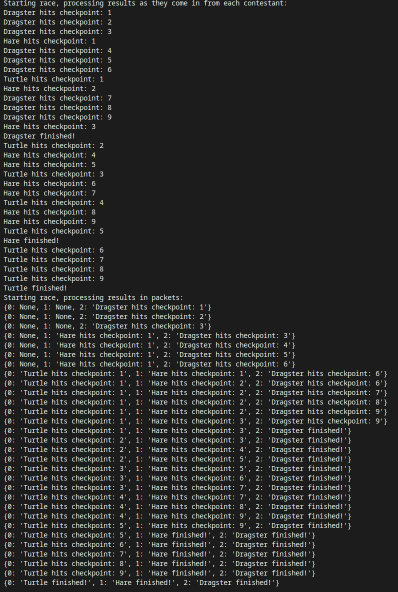
The whole point of this is that I wanted a way to combine the results of several concurrently running asynchronous generators as they come in, and, more importantly: identify exactly which result comes from which generator, without necessarily putting code in each specific generator to help with that identification. I wanted to keep the implementation of each algorithm focused on what it’s supposed to do and not tailor it to the fact that I want to use it in a scenario where I want to run several at the same time and compare them. That’s not a concern the algorithm needs to care for.
When you go and run the 4 different algorithms that will look for a solution to the TSP, you want to receive updates whenever some improvement is reached, or whenever something useful can be put on the screen, without polluting the generators with some identifying code to update the right result set. So the way it’s done in process_results_packet will be the method to use for running the 4 TSP algorithms together. I’ll just put the 4 algorithms in an array, start them all at the same time, and every time any one of them yields a result, I get a dictionary back with the updated results. It’s these few lines that do the trick:
    zipped = stream.ziplatest(*races)
    merged = stream.map(zipped, lambda x: dict(enumerate(x)))
    async with merged.stream() as streamer:
        ...
Quite simple and quite powerful. Ok, let’s get to the interesting parts now!
A brute force approach
Whenever you start implementing a non-trivial algorithm, it’s always a good idea to start with an implementation that is focused on getting the correct result, disregarding any tendency you might have to go for early optimizations. Make it as simple and clear as you can, but focus on achieving a 100% correct solution. Explore the full set of possible solutions, perform an exhaustive search and simply keep updating the candidate solution every time there’s an improvement until there are no more candidate solutions, and you just found yourself the optimal solution. It will help you understand the problem, and you can use this initial iteration as a reference to compare future solutions to, and doublecheck them for correctness.
In case of the TSP, implementing a brute-force solution is quite easy. We simply generate all possible permutations of the set of destinations, evaluate the full path distance from start through all nodes back to the initial node, and store the optimal path length and the sequence of nodes traveled in order to achieve it. Contrary to what I just said a sentence or two ago, I’d say some small optimizations are permitted. One such obvious thing is that a sequence of A - B - C - A is identical in length to the sequence A - C - B - A, and as such, both do not need to be evaluated. We only consider unique permutations. We obviously don’t need to continuously build the actual graph under consideration for the algorithm to work. However, I wanted to display the paths under evaluation as the algorithm does its work, so that little bit of extra effort is worth it for this project.
If you check the clip I linked before, you will see that during each iteration, a new path permutation (the lines in white) is being evaluated. Whenever a path is shorter than the known shortest path, that path is updated and shown in green. If you want to follow along with a bit more detail, just change the sleeping time at the end of the for-loop to something that gives you a bit more time to realize what’s occurring.
async def brute_force(graph: Graph, distances: dict[tuple[int, int], int]) -> AsyncIterator[AlgorithmResult]:
    """Solve the TSP problem with a brute force implementation, running through all permutations"""
    unique_permutations = set()
    paths_evaluated = 0
    evaluations_until_solved = 0
    start = graph[0].key
    keys = list(graph.nodes.keys())
    sub_keys = keys[1:]
    for permutation in permutations(sub_keys):
        permutation = (start,) + permutation + (start,)
        if permutation not in unique_permutations and permutation[::-1] not in unique_permutations:
            paths_evaluated += 1
            unique_permutations.add(permutation)
            current_path_length = 0
            node = start
            vertices: list[tuple[int, int, int]] = []
            for key in permutation[1:]:
                distance = distances[(node, key)]
                current_path_length += distance
                vertices.append((node, key, distance))
                node = key

            graph.remove_vertices()
            graph.add_vertices(vertices)
            if current_path_length < graph.optimal_cycle_length:
                graph.optimal_cycle = ShortestPath(current_path_length, vertices)
                evaluations_until_solved = paths_evaluated
            await asyncio.sleep(0.0001)
            yield AlgorithmResult(paths_evaluated, evaluations_until_solved)

    graph.remove_vertices()
    graph.add_vertices(graph.optimal_cycle.vertices)
    yield AlgorithmResult(paths_evaluated, evaluations_until_solved)
And there you have it. Problem solved! Well, kind of. For an ideal path between, let’s say, 5 or so points, I guess this brute force approach is still ok. You’ll notice, though, that when you have 8 or more points, things become very painful. Since we check all permutations, the runtime of the brute force algorithm is N! since we want to consider every possible vertex between each pair of nodes. Quite horrific, but at least we now have a way to test other, more optimal solutions for correctness.
Dynamic programming to the rescue
That brings us to an approach we’ve all used as a first optimization for so many algorithmic problems: dynamic programming. That will bring the time complexity down from O(n!) to O(n²2n). For the more curious readers that couldn’t help but scroll down instead of reading this, you’ve noticed that this requires quite a bit more code than our naive brute force approach. This already hammers home the statement about not diving into optimization too early. It’s easy to make a small mistake, and depending on how involved a solution you start to implement beyond brute force tactics, it can be quite cumbersome to debug.
The specific implementation I went for is one such example. As often the case when using dynamic programming, memoization is a big help here. But not only that, you also notice some bit-wise operations going on to further improve the speed of this solution. I will explain the steps we go through in this approach as best I can.
The overall approach here is that we will no longer consider all possible full paths through the set of nodes until we find the shortest one. As we do in dynamic programming, we solve a subset of the problem and keep expanding on it until we find a solution to the full problem. During this expansion, we use previously achieved results to avoid doing double work, using memoization. Here’s the full code (for all you copy-paste problem solvers out there 😉), read through it, and then I’ll focus on some specific parts. Just in case dynamic programming is a new concept to you, check out some articles or video tutorials online, maybe comparing greedy algorithms to dynamic programming for problems like the knapsack problem or coin change problem. That should help you get it down. The full code:
async def dynamic_programming(graph: Graph, distances: dict[tuple[int, int], int]
                              ) -> AsyncIterator[AlgorithmResult]:
    """Solve the TSP problem with dynamic programming"""
    node_count = len(graph)
    start = graph[0].key
    memo = [[0 for _ in range(1 << node_count)] for __ in range(node_count)]
    optimal_cycle = []
    optimal_cycle_length = maxsize
    cycles_evaluated = 0
    evaluations_until_solved = 0
    memo = setup(memo, graph, distances, start)
    for nodes_in_subcycle in range(2, node_count + 1):
        for subcycle in initialize_combinations(nodes_in_subcycle, node_count):
            if is_not_in(start, subcycle):
                continue

            cycles_evaluated += 1
            # Look for the best next node to attach to the cycle
            for next_node in range(node_count):
                if next_node == start or is_not_in(next_node, subcycle):
                    continue

                subcycle_without_next_node = subcycle ^ (1 << next_node)
                min_cycle_length = maxsize
                for last_node in range(node_count):
                    if (last_node == start or last_node == next_node or is_not_in(last_node, subcycle)):
                        continue

                    new_cycle_length = (memo[last_node][subcycle_without_next_node] + distances[(last_node, next_node)])
                    if new_cycle_length < min_cycle_length:
                        min_cycle_length = new_cycle_length
                    memo[next_node][subcycle] = min_cycle_length

        evaluations_until_solved = cycles_evaluated
        optimal_cycle_length = calculate_optimal_cycle_length(start, nodes_in_subcycle, memo, distances)
        optimal_cycle = find_optimal_cycle(start, nodes_in_subcycle, memo, distances)
        vertices = create_vertices(optimal_cycle, distances)
        graph.optimal_cycle = ShortestPath(optimal_cycle_length, vertices)
        await asyncio.sleep(0.0001)
        yield AlgorithmResult(cycles_evaluated, evaluations_until_solved)

    optimal_cycle_length = calculate_optimal_cycle_length(start, node_count, memo, distances)
    optimal_cycle = find_optimal_cycle(start, node_count, memo, distances)
    vertices = create_vertices(optimal_cycle, distances)
    graph.remove_vertices()
    graph.add_vertices(vertices)
    graph.optimal_cycle = ShortestPath(optimal_cycle_length, vertices)
    yield AlgorithmResult(cycles_evaluated, evaluations_until_solved)


def setup(memo: list, graph: Graph, distances: dict[tuple[int, int], int], start: int) -> list:
    """Prepare the array used for memoization during the dynamic programming algorithm"""
    for i, node in enumerate(graph):
        if start == node.key:
            continue

        memo[i][1 << start | 1 << i] = distances[(start, i)]

    return memo


def initialize_combinations(nodes_in_subcycle: int, node_count: int) -> list[int]:
    """Initialize the combinations to consider in the next step of the algorithm"""
    subcycle_list = []
    initialize_combination(0, 0, nodes_in_subcycle, node_count, subcycle_list)

    return subcycle_list


def initialize_combination(subcycle, at, nodes_in_subcycle, node_count, subcycle_list) -> None:
    """Initialize the combination to consider in the next step of the algorithm"""
    elements_left_to_pick = node_count - at
    if elements_left_to_pick < nodes_in_subcycle:
        return

    if nodes_in_subcycle == 0:
        subcycle_list.append(subcycle)
    else:
        for i in range(at, node_count):
            subcycle |= 1 << i
            initialize_combination(subcycle, i + 1, nodes_in_subcycle - 1,
                                   node_count, subcycle_list)
            subcycle &= ~(1 << i)


def is_not_in(index, subcycle) -> bool:
    """Checks if the bit at the given index is a 0"""
    return ((1 << index) & subcycle) == 0


def calculate_optimal_cycle_length(start: int, node_count: int, memo: list,
                                   distances: dict[tuple[int, int], int]) -> int:
    """Calculate the optimal cycle length"""
    end = (1 << node_count) - 1
    optimal_cycle_length = maxsize
    for i in range(node_count):
        if i == start:
            continue

        cycle_cost = memo[i][end] + distances[(i, start)]
        if cycle_cost < optimal_cycle_length:
            optimal_cycle_length = cycle_cost

    return optimal_cycle_length


def find_optimal_cycle(start: int, node_count: int, memo: list,
                       distances: dict[tuple[int, int], int]):
    """Recreate the optimal cycle"""
    last_index = start
    state = (1 << node_count) - 1
    optimal_cycle: list[int] = []
    for _ in range(node_count - 1, 0, -1):
        index = -1
        for j in range(node_count):
            if j == start or is_not_in(j, state):
                continue

            if index == -1:
                index = j
            prev_cycle_length = memo[index][state] + distances[(index, last_index)]
            new_cycle_length = memo[j][state] + distances[(j, last_index)]
            if new_cycle_length < prev_cycle_length:
                index = j

        optimal_cycle.append(index)
        state = state ^ (1 << index)
        last_index = index
    optimal_cycle.append(start)
    optimal_cycle.reverse()
    optimal_cycle.append(start)

    return optimal_cycle


def create_vertices(optimal_cycle: list[int], distances: dict[tuple[int, int], int]
                    ) -> list[tuple[int, int, int]]:
    """Transform the list of visited node keys to something our graph can work with"""
    vertices: list[tuple[int, int, int]] = []
    for i in range(1, len(optimal_cycle)):
        weight = distances[(optimal_cycle[i - 1], optimal_cycle[i])]
        vertices.append((optimal_cycle[i - 1], optimal_cycle[i], weight))

    return vertices
Again, in case you want to understand the steps at a high level, change the sleep time to about a second or so, and you will see what happens. Starting with a cycle of 2 nodes, building up to a cycle including all the points, we find the shortest possible path using the points we include in the cycle. Whenever an optimal solution is found for 2 points, we find an optimal solution for those 2 points plus 1 more, reusing what we have already learned so far. We keep doing that until the full set of nodes has been traveled. It’s really quite beautiful to see in action, in my opinion. How to achieve it, though?
Getting the memoization matrix set up
We start out by preparing our memoization matrix:
memo = [[0 for _ in range(1 << node_count)] for __ in range(node_count)]
...
def setup(memo: list, graph: Graph, distances: dict[tuple[int, int], int], start: int) -> list:
    for i, node in enumerate(graph):
        if start == node.key:
            continue

        memo[i][1 << start | 1 << i] = distances[(start, i)]

    return memo
Here, I create a matrix with a number of rows equal to the number of nodes we have and columns equal to 2 raised to the power of the number of nodes. So for 5 nodes, that’s a 5x32 matrix. As you may know, raising 2 to the power of N equals shifting a 1-bit to the left N times, since a move to the left doubles the binary value. It’s just faster using bit shifting, simple as that. We loop through each node, skipping the start node, and we store the optimal distance from the start node to each other node.
Other helper functions
Besides the preparation of the memoization matrix, other functions such as find_optimal_cycle and create_vertices are actually not terribly complicated or interesting. If we keep in mind that, during dynamic programming, we build on top of earlier achieved results (optimal paths through n nodes) to get the optimal result for n+1 nodes, it’s not hard to imagine we will need to consider a new set of cycles and nodes to evaluate whether adding a certain node to our cycle yields a more optimal results than adding another. Beyond that, in the visualization of the brute force algorithm ,you noticed we kept on drawing the vertices under consideration. For the dynamic programming solution, we simply want to build the new optimal cycle and put it on the screen, so we have some functions for that. Stepping through them with a small number of nodes will make it very clear what they do. Be sure to brush off those bit manipulator operations first 😉
Just one more thing
Maybe a bit of explanation on the initialize_combinations and initialize_combination methods: initialize_combinations will fill the subcycle_list variable using the initialize_combination method, that much is obvious. initialize_combination is a recursive method to generate bit sets, starting from an empty set (0). From an empty set, we want to set nodes_in_subcycle out of node_count bits to be 1 for all possible combinations. We keep track of which index position we’re at (indicated by variable i), try to set it to 1 and keep moving forward. At the end of that, we should have exactly node_count bits. If we don’t, we backtrack and flip off (not like that) the i-th bit and move to the next position. This is a classic backtracking problem, and if you want to learn more about it, look for backtracking tutorials for power sets.
def initialize_combinations(nodes_in_subcycle: int, node_count: int) -> list[int]:
    """Initialize the combinations to consider in the next step of the algorithm"""
    subcycle_list = []
    initialize_combination(0, 0, nodes_in_subcycle, node_count, subcycle_list)

    return subcycle_list


def initialize_combination(subcycle, at, nodes_in_subcycle, node_count, subcycle_list) -> None:
    """Initialize the combination to consider in the next step of the algorithm"""
    elements_left_to_pick = node_count - at
    if elements_left_to_pick < nodes_in_subcycle:
        return

    if nodes_in_subcycle == 0:
        subcycle_list.append(subcycle)
    else:
        for i in range(at, node_count):
            subcycle |= 1 << i
            initialize_combination(subcycle, i + 1, nodes_in_subcycle - 1,
                                   node_count, subcycle_list)
            subcycle &= ~(1 << i)
Solving the puzzle
This is where the actual work happens, and there’s a bit to it. Make sure the other functions are clear to you and the use of a memoization matrix in dynamic programming in general is a concept you understand.
    for nodes_in_subcycle in range(2, node_count + 1):
        for subcycle in initialize_combinations(nodes_in_subcycle, node_count):
            if is_not_in(start, subcycle):
                continue

            cycles_evaluated += 1
            # Look for the best next node to attach to the cycle
            for next_node in range(node_count):
                if next_node == start or is_not_in(next_node, subcycle):
                    continue

                subcycle_without_next_node = subcycle ^ (1 << next_node)
                min_cycle_length = maxsize
                for last_node in range(node_count):
                    if (last_node == start or last_node == next_node or is_not_in(last_node, subcycle)):
                        continue

                    new_cycle_length = (memo[last_node][subcycle_without_next_node] + distances[(last_node, next_node)])
                    if new_cycle_length < min_cycle_length:
                        min_cycle_length = new_cycle_length
                    memo[next_node][subcycle] = min_cycle_length

        evaluations_until_solved = cycles_evaluated
        optimal_cycle_length = calculate_optimal_cycle_length(start, nodes_in_subcycle, memo, distances)
        optimal_cycle = find_optimal_cycle(start, nodes_in_subcycle, memo, distances)
        vertices = create_vertices(optimal_cycle, distances)
        graph.optimal_cycle = ShortestPath(optimal_cycle_length, vertices)
        await asyncio.sleep(0.0001)
        yield AlgorithmResult(cycles_evaluated, evaluations_until_solved)
As you can see, the outer loop increases the length of the cycle by 1 with each iteration. In every iteration, we find the optimal cycle of a certain length, increasing the cycle length until we have an optimal cycle equal to the number of nodes. The first inner loop goes over all the distinct subcycles we want to consider. Obviously, we only want to consider subcycles where the start node is actually part of the subcycle. Otherwise, that subcycle could not have started at the starting node. The function to check that is called is_not_in (I know it’s a one-line function… in my defense, there’s a npm package called “is_even”. So hold your horses 😀):
def is_not_in(index, subcycle) -> bool:
    """Checks if the bit at the given index is a 0"""
    return ((1 << index) & subcycle) == 0
and all that’s done here is check whether or not the bit at the index position in the subcycle is a 0. If it is, the node is not part of the subcycle.
After that, we loop over all the potential next nodes. Here, we only want to consider nodes that are actually in the subcycle and are not equal to our starting node. We then represent the next subcycle without this next node. We do this so we can use our memoization matrix to look up what the best partial tour length was without the next node already included. The last inner loop, where we cycle the last_node variable over the range of possible nodes, is there to test all possible end nodes of the currently considered subcycle, and consider which node best optimizes that subcycle. This last node can, of course, not be the start node or the next node that is fixed in the loop before and should be part of the current subcycle.
Per potential new last node, we check if the cost of the cycle with this last node is better than the currently known lowest cost (or shortest distance in our case). If so, we set the new min_cycle_length and store the best subcycle in the memoization matrix.
At the end of each new subcycle length, we do some bookkeeping and a little bit of work to reconstruct the actual newly found shortest cycle of length nodes_in_subcycle and yield that back so it can be displayed on screen. The functions calculate_optimal_cycle_length and find_optimal_cycle are responsible for this. If you are familiar with dynamic programming, reconstructing a solution from a memoization table will be familiar to you. The only bit of added complexity here is that this reconstruction is done using our bitmasks in the memoization table.
And that does it. If this is not entirely clear, I recommend you make sure the basics of dynamic programming and bit-wise operators are under your belt, and simply step through the code using a graph with 5 or so nodes. That allows you to still reason about the whole concept and actually follow along what is happening.
Beware Python looping
A final word of warning if you play around with this yourself: there’s quite a bit of looping going on in this implementation. Normally, that would be no issue. Python, however, is notoriously slow when it comes to looping. In my previous post about the Game of Life, I tackled that problem by using Numpy, Numba, and some search space optimizations. I decided not to take that route this time, however, since I didn’t want to make the implementation even more complex, and also give a fair comparison of all 4 algorithms without any trickery going into it. I will probably make a Rust 🦀 version at some point, probably without too many visuals going on (unless I get good at Bevy real fast), so the raw performance potential of several algorithms is more obvious. For now, though, bear with me (or Python, rather). I don’t execute the brute force and dynamic programming algorithms when the number of nodes exceeds 8 and 17 nodes, respectively, so things won’t be overly painful.
Genetic algorithm
Finally, this is where the real fun starts… Now that we have two ways of solving the TSP that give us a guaranteed optimal result, even though it might take a bit to get there, we’ll dig into some approximation algorithms. Firstly, genetic algorithms. You will see that the code isn’t terribly complex at all, which allows me to focus on the high-level concepts of these interesting algorithms and apply them to this problem. If the dynamic programming section was a bit of a head-scratcher, no worries; it’s all fun and games from here on out.
Genetic? Evolution?
First and foremost, what are genetic algorithms..? They are an optimization technique, using concepts from evolutionary biology to search for a global optimal solution. As you would expect when drawing the analogy to evolution, we start with an initial population. We will crossbreed certain entities from the population with each other to obtain a new generation. There are various techniques we can apply to this process, and as you would expect, strong specimens will be more likely to breed, and some random mutations will also occur. As such, it really mimics the process of evolutionary biology, where we have non-random survival, with non-random selection, and random mutation. The survival of a certain specimen (or the spreading of its ‘genes) is steered by a fitness function that measures how well it can optimize for its purpose (in our case, finding the shortest route between a set of nodes). Stronger specimens have a higher chance of propagating their DNA through the generations, as they are more likely to be chosen for reproduction. To make sure there is some sense of discovery built into the whole system, random mutation will be an important part of the process.
When I first read about these algorithms, I got incredibly excited to learn about them, take a swing at them myself, and I’m still amazed at how well the whole concept works. You will see that close to optimal results can be achieved very quickly, both in terms of generations needed to do so and in terms of processing time. Each step is fairly simple, very visual, and easy to implement. Most of the difficulty regarding the efficacy of these algorithms lies in the details and many of the parameters. How big is my population? How many generations will I evolve before I stop and accept the result as close enough to optimal? What techniques will I use to steer the crossbreeding? How will I introduce genetic mutations in new specimens? A lot of these questions are often a matter of experimentation. Since I’m still very much a beginner in terms of these algorithms, I’d encourage you to start your own learning journey if all of this spikes your interest. For now, let me show you the implementation I came up with after experimenting with all of the above:
async def genetic_algorithm(graph: Graph, distances: dict[tuple[int, int], int], population_size: int,
                            max_generations: int, max_no_improvement: int) -> AsyncIterator[AlgorithmResult]:
    """Solve the TSP problem with a genetic algorithm"""
    generations_evaluated = 0
    generations_until_solved = 0
    generations_without_improvement = 0
    optimal_cycle: list[int] = []
    optimal_cycle_length = maxsize
    population = spawn(graph, population_size)
    cycle_lengths = get_cycle_lengths(population, distances)
    for _ in range(max_generations):
        if generations_without_improvement >= max_no_improvement:
            break

        fitness = determine_fitness(cycle_lengths)
        improved = False
        for i, cycle_length in enumerate(cycle_lengths):
            if cycle_length < optimal_cycle_length:
                improved = True
                optimal_cycle_length = cycle_length
                optimal_cycle = population[i]

        generations_evaluated += 1
        if improved:
            generations_until_solved = generations_evaluated
            generations_without_improvement = 0
            vertices: list[tuple[int, int, int]] = []
            node = optimal_cycle[0]
            for key in optimal_cycle[1:]:
                distance = distances[(node, key)]
                vertices.append((node, key, distance))
                node = key
            graph.remove_vertices()
            graph.add_vertices(vertices)
            graph.optimal_cycle = ShortestPath(optimal_cycle_length, vertices)
        else:
            generations_without_improvement += 1

        if len(population) == 1:
            break
        population, cycle_lengths = create_next_population(population, cycle_lengths,
                                                           fitness, distances)
        await asyncio.sleep(0.0001)
        yield AlgorithmResult(generations_evaluated, generations_until_solved)
    yield AlgorithmResult(generations_evaluated, generations_until_solved)


def spawn(graph: Graph, population_size: int) -> list[list[int]]:
    """Create the initial generation"""
    start = graph[0].key
    keys = list(graph.nodes.keys())[1:]
    max_size = int(factorial(len(keys)) / 2)
    unique_permutations = set()
    while len(unique_permutations) < population_size and len(unique_permutations) < max_size:
        permutation = list(keys)
        shuffle(permutation)
        permutation = (start,) + tuple(permutation) + (start,)
        if permutation[::-1] not in unique_permutations:
            unique_permutations.add(permutation)

    return [list(permutation) for permutation in unique_permutations]


def create_next_population(current_population: list[list[int]], cycle_lengths: list[int],
                           fitness: list[float], distances: dict[tuple[int, int], int]
                           ) -> tuple[list[list[int]], list[int]]:
    """Create the next generation"""
    new_population: list[list[int]] = []
    population_size = len(current_population)

    # Create the offspring of the current generation
    offspring = create_offspring(current_population, fitness, population_size)

    # Perform a variation of elitism where we add the offspring to the current generation
    # and only continue with the fittest list of size population_size
    new_population = current_population + offspring
    offspring_cycle_lengths = get_cycle_lengths(offspring, distances)
    new_population_cycle_lengths = cycle_lengths + offspring_cycle_lengths
    new_population_fitness = fitness + determine_fitness(offspring_cycle_lengths)
    survivor_candidates = zip(new_population_fitness, new_population)
    fittest_indices = [i for _, i in heapq.nlargest(population_size, ((x, i) for i, x in enumerate(survivor_candidates)))]
    new_population = [new_population[i] for i in fittest_indices]
    new_population_cycle_lengths = [new_population_cycle_lengths[i] for i in fittest_indices]

    return new_population, new_population_cycle_lengths


def create_offspring(current_population: list[list[int]], fitness: list[float],
                     population_size: int) -> list[list[int]]:
    """Create a new generation"""
    offspring: list[list[int]] = []
    while len(offspring) < population_size:
        parent1 = parent2 = 0
        while parent1 == parent2:
            parent1 = get_parent(fitness)
            parent2 = get_parent(fitness)

        child1 = crossover(current_population[parent1], current_population[parent2])
        child2 = crossover(current_population[parent2], current_population[parent1])

        child1 = mutate(child1)
        child2 = mutate(child2)

        offspring.append(child1)
        offspring.append(child2)

    return offspring


def get_parent(fitness: list[float]):
    """Get a parent using either tournament selection or biased random selection"""
    if randint(0, 1):
        return tournament_selection(fitness)

    return biased_random_selection(fitness)


def tournament_selection(fitness: list[float]) -> int:
    """Perform basic tournament selection to get a parent"""
    start, end = 0, len(fitness) - 1
    candidate1 = randint(start, end)
    candidate2 = randint(start, end)
    while candidate1 == candidate2:
        candidate2 = randint(start, end)

    return candidate1 if fitness[candidate1] > fitness[candidate2] else candidate2


def biased_random_selection(fitness: list[float]) -> int:
    """Perform biased random selection to get a parent"""
    random_specimen = randint(0, len(fitness) - 1)
    for i, _ in enumerate(fitness):
        if fitness[i] >= fitness[random_specimen]:
            return i

    return random_specimen


def crossover(parent1: list[int], parent2: list[int]) -> list[int]:
    """Cross-breed a new set of children from the given parents"""
    start = parent1[0]
    end = parent1[len(parent1) - 1]
    parent1 = parent1[1:len(parent1) - 1]
    parent2 = parent2[1:len(parent2) - 1]
    split = randint(1, len(parent1) - 1)
    child: list[int] = [0] * len(parent1)
    for i in range(split):
        child[i] = parent1[i]

    remainder = [i for i in parent2 if i not in child]
    for i, data in enumerate(remainder):
        child[split + i] = data

    return [start, *child, end]


def mutate(child: list[int]) -> list[int]:
    """Mutate the child sequence"""
    if randint(0, 1):
        child = swap_mutate(child)
    child = rotate_mutate(child)

    return child


def swap_mutate(child: list[int]) -> list[int]:
    """Mutate the cycle by swapping 2 nodes"""
    index1 = randint(1, len(child) - 2)
    index2 = randint(1, len(child) - 2)
    child[index1], child[index2] = child[index2], child[index1]

    return child


def rotate_mutate(child: list[int]) -> list[int]:
    """Mutate the cycle by rotating a part nodes"""
    split = randint(1, len(child) - 2)
    head = child[0:split]
    mid = child[split:len(child) - 1][::-1]
    tail = child[len(child) - 1:]
    child = head + mid + tail

    return child


def get_cycle_lengths(population: list[list[int]],
                      distances: dict[tuple[int, int], int]) -> list[int]:
    """Get the lengths of all cycles in the graph"""
    cycle_lengths: list[int] = []
    for specimen in population:
        node = specimen[0]
        cycle_length = 0
        for key in specimen[1:]:
            key = int(key)
            cycle_length += distances[(node, key)]
            node = key
        cycle_lengths.append(cycle_length)

    return cycle_lengths


def determine_fitness(cycle_lengths: list[int]) -> list[float]:
    """Determine the fitness of the specimens in the population"""
    # Invert so that shorter paths get higher values
    fitness_sum = sum(cycle_lengths)
    fitness = [fitness_sum / cycle_length for cycle_length in cycle_lengths]

    # Normalize the fitness
    fitness_sum = sum(fitness)
    fitness = [f / fitness_sum for f in fitness]

    return fitness
The initial population
If you take your time to go over the implementation and maybe step through it yourself, I think your first impression will be that the complexity here is fairly low. Let’s go over what exactly happens, and focus on some of the functions in detail. Our first task is to spawn an initial population:
population = spawn(graph, population_size)
...
def spawn(graph: Graph, population_size: int) -> list[list[int]]:
    """Create the initial generation"""
    start = graph[0].key
    keys = list(graph.nodes.keys())[1:]
    max_size = int(factorial(len(keys)) / 2)
    unique_permutations = set()
    while len(unique_permutations) < population_size and len(unique_permutations) < max_size:
        permutation = list(keys)
        shuffle(permutation)
        permutation = (start,) + tuple(permutation) + (start,)
        if permutation[::-1] not in unique_permutations:
            unique_permutations.add(permutation)

    return [list(permutation) for permutation in unique_permutations]
So what does it mean to have a “population”? For our particular problem, each specimen in the population is basically a candidate route that starts out at our designated starting node, visits every other node exactly once, and arrives back at that starting node. Whether or not that’s an optimal route or not is of no significance at this point. We trust that an approximation of the ideal route can be achieved through evolution, and we won’t have to perform an exhaustive search through all permutations. That last part is the whole point of it, especially for problems that are NP-hard: we do not want to generate the full set of potential solutions and go through them one by one. We will simply generate a number of candidate solutions and start the process from there. Also, it’s important that these initial candidate solutions be chosen randomly. When we use heuristics to already pre-optimize candidates, this leads to low diversity in the population, which can yield suboptimal solutions. There is no need to increase the initial fitness of the population. It’s the diversity of the solutions that will lead to optimality.
That begs another question: how do we determine the size of our initial population? If we start with a high initial population count, this can cause the algorithm to perform very poorly, which we want to avoid. Then again, an overly small population may not be enough to create a high-quality and diverse mating pool. A lot of trial and error can go into finding a population size that suits the specific problem. In this case, I have settled on half of n!, where n is the set of nodes excluding the starting node. For example, if we have a set of 8 total nodes, the initial population size would consist of (7!) / 2 = 2520. Putting it in perspective, in this case, there would be 40320 potential solutions, so we’re still far from generating the full set of candidates. In case you want to learn more, there are several whitepapers out there that just focus on techniques to determine the ideal initial population size.
Keep on spinning forever?
So now that we have decided on an initial population, the next question is: how long will we keep this little ecosystem doing its thing? Remember two sentences back? Yeah, there’s also enough research going on regarding that question. At some point, there is simply no improvement possible since we converged on the optimal solution, or the whole cycle doesn’t yield any improvement anymore. Since we’ll never know whether we actually found an optimal solution (not without some “help” from the outside at least), we’ll just decide to stop running the algorithm when we haven’t seen any improvement for a certain number of generations:
    for _ in range(max_generations):
        if generations_without_improvement >= max_no_improvement:
            break
What that number is will be dependent on the size of the problem and many other factors. In main.py, you see that some experimentation made me settle on some numbers of population size and max_generations that seemed to work well for a certain number of nodes:
    def __determine_ga_parameters(self, node_count: int) -> tuple[int, int]:
        match node_count:
            case _ if node_count <= 5: return 50, 5
            case _ if node_count <= 10: return 250, 10
            case _ if node_count <= 15: return 500, 30
            case _ if node_count <= 20: return 750, 50
            case _ if node_count <= 25: return 1000, 75
            case _ if node_count <= 30: return 1250, 100
            case _ if node_count <= 35: return 1500, 150
            case _ if node_count <= 50: return 5000, 250
        return 25000, 500
Nature calls
And after that, you could say it’s off to the races. We first determine the fitness of our current population, which is fairly simple. All we do is take the total sum of the cycle lengths and divide the length of each cycle by that number. That way, shorter paths get higher values. We then just normalize those values so they all sum up to 1.
def determine_fitness(cycle_lengths: list[int]) -> list[float]:
    """Determine the fitness of the specimens in the population"""
    # Invert so that shorter paths get higher values
    fitness_sum = sum(cycle_lengths)
    fitness = [fitness_sum / cycle_length for cycle_length in cycle_lengths]

    # Normalize the fitness
    fitness_sum = sum(fitness)
    fitness = [f / fitness_sum for f in fitness]

    return fitness
After this step, we check if we found a shorter cycle in this generation and update the shortest known cycle to that specific candidate. We then do some bookkeeping to update our graph to reflect this newly found solution, which is just something we do for this particular project in order to display intermediary results. The next important thing we need to do is create a whole new generation. There are a lot of possibilities to experiment with here, from the methods for selection to the way we introduce mutation, and even the size of the new population.
Non-random selection
What determines which specimens get to propagate their DNA through the generations? The temptation might be to simply select only the strongest candidate solutions. This will inevitably lead to getting stuck in local optimal solutions, low diversity in the population, and ultimately, far from a close-to-optimal solution in the long run. There are two quite popular methods for selecting parents: tournament selection and biased random selection. We will randomly select either one of them. If you think: “that sounds awefully random to me; where does the non-random part come in?” no worries, both still favor more fit specimens.
Tournament selection works as follows: we pick two completely random candidate solutions out of the population, and whichever has the highest fitness wins. Yeah. That’s it. I told you the code was simple. Here it is:
def tournament_selection(fitness: list[float]) -> int:
    """Perform basic tournament selection to get a parent"""
    start, end = 0, len(fitness) - 1
    candidate1 = randint(start, end)
    candidate2 = randint(start, end)
    while candidate1 == candidate2:
        candidate2 = randint(start, end)

    return candidate1 if fitness[candidate1] > fitness[candidate2] else candidate2
As an alternative, biased random selection works a bit differently. We select a random specimen, and we look for the first specimen in the list that has a higher fitness score than that random one. If we find it. If not, the initially randomly selected specimen is the one that will return. Quite literally random, but… biased.
def biased_random_selection(fitness: list[float]) -> int:
    """Perform biased random selection to get a parent"""
    random_specimen = randint(0, len(fitness) - 1)
    for i, _ in enumerate(fitness):
        if fitness[i] >= fitness[random_specimen]:
            return i

    return random_specimen
Crossover
Great, so now we have two parents. We all know what comes next. Detail: we don’t have to limit ourselves to only 2 parents in the case of crossover during genetic algorithms, there’s no reason why we would not use 3/4 or more parents when creating a new specimen for the next generation (also, wipe that smirk off your face). In this case, let’s be nice about it and stick to two parents. Our crossover function looks as follows:
def crossover(parent1: list[int], parent2: list[int]) -> list[int]:
    """Cross-breed a new set of children from the given parents"""
    start = parent1[0]
    end = parent1[len(parent1) - 1]
    parent1 = parent1[1:len(parent1) - 1]
    parent2 = parent2[1:len(parent2) - 1]
    split = randint(1, len(parent1) - 1)
    child: list[int] = [0] * len(parent1)
    for i in range(split):
        child[i] = parent1[i]

    remainder = [i for i in parent2 if i not in child]
    for i, data in enumerate(remainder):
        child[split + i] = data

    return [start, *child, end]
“A part of mommy, a part of dad”. It sounds clumsily simple, but that is really all there is to it. We take a part of the first parent and assign it to our offspring. That “part”, in case you are wondering, is just the start of the route as described by the parent specimen. A certain sequence of nodes, starting from our designated starting node, up to some cut-off point that is randomly decided on. That is basically our DNA. After this, we need to complete the route from the cut-off point back to the starting node. In this case, though, we need to respect the problem at hand and make sure we only visit each node once. So we loop through the nodes of parent2 and only add each node to the child if it has not been visited yet. You could say that potentially scrambles up the second part of the offspring candidate, and that is true. We literally take the exact sequence of nodes of parent1 up to the cut-off point but will not respect the sequence of nodes of parent2 as we add them to the child.
Mutation
As we all know, biology isn’t perfect, so let’s include some random mutations just like they happen in nature. After generating our offspring per parent pair, we mutate them using one of two possible methods. Swap mutate, and rotate mutate. Why introduce mutations at all? We want to maintain genetic diversity in our population so we don’t get stuck in local mimima. Usually, in genetic algorithms, mutation is only done sporadically. Here, you see that I mutate every single offspring specimen. Experiment yourself when implementing genetic algorithms for your specific problem to see what works and what doesn’t.
Swap mutate is a really simple and low-impact mutation that will simply swap 2 nodes in the sequence, and it looks like this:
def swap_mutate(child: list[int]) -> list[int]:
    """Mutate the cycle by swapping 2 nodes"""
    index1 = randint(1, len(child) - 2)
    index2 = randint(1, len(child) - 2)
    child[index1], child[index2] = child[index2], child[index1]

    return child
On the other hand, rotate mutation really scrambles up the specimen. We chose a split point, excluding the start node, and divided our sequence into a head, mid, and tail. We then completely reversed the mid, and reconstruct the sequence. This adds quite some diversity to the population.
def rotate_mutate(child: list[int]) -> list[int]:
    """Mutate the cycle by rotating a part nodes"""
    split = randint(1, len(child) - 2)
    head = child[0:split]
    mid = child[split:len(child) - 1][::-1]
    tail = child[len(child) - 1:]
    child = head + mid + tail

    return child
And that is all there is to it. As a reminder, the full create_offspring function, with all these building blocks put together, looks like this:
def create_offspring(current_population: list[list[int]], fitness: list[float],
                     population_size: int) -> list[list[int]]:
    """Create a new generation"""
    offspring: list[list[int]] = []
    while len(offspring) < population_size:
        parent1 = parent2 = 0
        while parent1 == parent2:
            parent1 = get_parent(fitness)
            parent2 = get_parent(fitness)

        child1 = crossover(current_population[parent1], current_population[parent2])
        child2 = crossover(current_population[parent2], current_population[parent1])

        child1 = mutate(child1)
        child2 = mutate(child2)

        offspring.append(child1)
        offspring.append(child2)

    return offspring
Now that we focused on each individual step, the complete function is very simple to understand. We simply keep pairing up two selected parents, create two children per parent, apply mutation to each of them, and add them to the new generation.
Let’s get fancy about it
Just one more thing, though. We did create a whole new generation of candidate solutions, equal in size to the previous generation. We introduced a bunch of randomization along the way, both in the selection of parents as well as in how their DNA was propagated to the next generation. And just like in nature, the parents have now played their parts, and they die a lonely death, assured in the knowledge that all that was best about them lives on in their children as they wither away. Wait, that got way too grim, way too fast. Also, this isn’t nature. Or is it? We’re still playing survival of the fittest, and there’s no need to brush aside our strong performers just because we’ve got a new generation waiting to take over.
So we’ll introduce another little technique called elitism, which is implemented as such:
    new_population = current_population + offspring
    offspring_cycle_lengths = get_cycle_lengths(offspring, distances)
    new_population_cycle_lengths = cycle_lengths + offspring_cycle_lengths
    new_population_fitness = fitness + determine_fitness(offspring_cycle_lengths)
    survivor_candidates = zip(new_population_fitness, new_population)
    fittest_indices = [i for _, i in heapq.nlargest(population_size, ((x, i) for i, x in enumerate(survivor_candidates)))]
    new_population = [new_population[i] for i in fittest_indices]
    new_population_cycle_lengths = [new_population_cycle_lengths[i] for i in fittest_indices]
We simply add the new generation of offspring to the current generation. And then we execute our fitness function again. If you’re a visual thinker, imagine we’re having ourselves a good old brawl that will knock out half of the population, leaving the strongest ones standing. It’s these specimens that we’ll keep on board to continue the algorithm. Also, notice we’re using a priority queue, which has a max binary heap implementation under the hood to only select the best x largest of elements without having to order the full list. I actually implemented that myself here - well it’s a min binary heap there, same idea though - before I knew that there was an implementation built-in 😉 Still, I strongly believe that you should know about and be able to implement these kinds of basic data structures on your own. Don’t depend on others to do all the thinking for you. I always valued fundamentals, algorithms, and data structures way more than cobbling together packages and frameworks. And it seems like, in these ChatGPT times where example implementations of frameworks are a prompt away, that’ll be even more useful than ever.
In any case, that’s all in terms of implementation. As I said before, the code isn’t really that involved at all, and each step can be easily visualized. This is only a very basic implementation, though, and there’s so much to uncover about genetic algorithms, techniques to perform crossover, selection, mutation, optimization of the parameters and so much more. I hope this small example does trigger your interest to start researching more about them. It’s really quite wonderful how such a simple concept can yield very good results in a short time.
Thousands of little creepers…
Talking about wonderful… The next algorithm got me even more excited than genetic algorithms. We’ll stick to nature, but switch gears from the wonders of evolution to the behavior of one of the most numerous animals on the planet: ants! I was extremely excited to dig my fingers into this one, and I hope it will get you equally excited. Ant colony optimization is a very interesting algorithm where we mimic the behavior of ant swarms. We will unleash a number of waves of ants onto our starting node and have them explore our graph until they visit all nodes and end up back at the starting node. As they explore the graph, they leave behind a pheromone trail that will encourage other ants to also take that route. The better (shorter, in our case) a route is, the stronger the pheromone trail, and the more chance there is that another ant will prefer to take that route, leaving behind additional pheromones to further strengthen that path. To also introduce some sense of exploration and to avoid local minima, pheromones will evaporate over time. While getting myself familiar with the overall concept and the details behind it, several clips of HK Lam, like this one and others helped my understanding tremendously. He has playlists on several interesting topics in the same sphere, definitely check them out! The full code of the algorithm:
async def ant_colony(graph: Graph, distances: dict[tuple[int, int], int],
                     max_swarms: int, max_no_improvement: int) -> AsyncIterator[AlgorithmResult]:
    """Solve the TSP problem using ant colony optimization"""
    swarms_evaluated = 0
    evaluations_until_solved = 0
    swarms_without_improvement = 0
    node_count = len(graph.nodes)
    pheromones = initialize_pheromones(node_count, distances)
    for _ in range(max_swarms):
        if swarms_without_improvement >= max_no_improvement:
            break

        vertices, cycle_lengths = swarm_traversal(pheromones, distances)
        pheromones = pheromone_evaporation(pheromones)
        best_cycle_index = np.argmin(cycle_lengths)
        best_cycle = vertices[best_cycle_index]
        best_cycle_length = cycle_lengths[best_cycle_index]
        pheromones = pheromone_release(vertices, best_cycle, best_cycle_length, pheromones)
        pheromones = normalize(pheromones)
        swarms_evaluated += 1

        if cycle_lengths[best_cycle_index] < graph.optimal_cycle_length:
            graph.remove_vertices()
            graph.add_vertices(best_cycle)
            graph.optimal_cycle = ShortestPath(best_cycle_length, best_cycle)
            evaluations_until_solved = swarms_evaluated
            swarms_without_improvement = 0
            await asyncio.sleep(0.0001)
            yield AlgorithmResult(swarms_evaluated, evaluations_until_solved)
        else:
            swarms_without_improvement += 1
    yield AlgorithmResult(swarms_evaluated, evaluations_until_solved)


def initialize_pheromones(node_count: int, distances: dict[tuple[int, int], int]) -> np.ndarray:
    """Initialize the pheromone array"""
    pheromones = np.zeros((node_count, node_count), dtype=float)
    for i, j in np.ndindex(pheromones.shape):
        if i != j:
            pheromones[i, j] = distances[(i, j)]
    for i in range(node_count):
        row_sum = sum(pheromones[i, :])
        for j in range(node_count):
            if i != j:
                pheromones[i, j] = row_sum / pheromones[i, j]
        row_sum = sum(pheromones[i, :])
        for j in range(node_count):
            if i != j:
                pheromones[i, j] /= row_sum
    return pheromones


def normalize(pheromones: np.ndarray) -> np.ndarray:
    """Normalize the pheromone matrix into probabilities"""
    node_count = pheromones.shape[0]
    for i in range(node_count):
        row_sum = sum(pheromones[i, :])
        for j in range(node_count):
            if i != j:
                pheromones[i, j] /= row_sum
    return pheromones


def swarm_traversal(pheromones: np.ndarray, distances: dict[tuple[int, int], int]) -> tuple[np.ndarray, list[int]]:
    """Traverse the graph with a number of ants equal to the number of nodes"""
    node_count = pheromones.shape[0]
    swarm_size = node_count * node_count
    vertices = np.array([[(0, 0, 0)] * node_count] * swarm_size, dtype="i,i,i")
    cycle_lengths: list[int] = [0] * swarm_size
    # Traverse the graph swarm_size times
    with ThreadPoolExecutor(max_workers=min(swarm_size, 50)) as executor:
        futures = [executor.submit(traverse, node_count, pheromones, distances)
                   for i in range(swarm_size)]
        for i, completed in enumerate(as_completed(futures)):
            cycle_length, cycle = completed.result()
            vertices[i] = cycle
            cycle_lengths[i] = cycle_length
    return vertices, cycle_lengths


def traverse(node_count: int, pheromones: np.ndarray,
             distances: dict[tuple[int, int], int]) -> tuple[int, np.ndarray]:
    """Perform a traversal through the graph"""
    # Each traversal consists of node_count vertices
    current_node = 0
    visited = set([current_node])
    cycle_length = 0
    vertices = np.array([(0, 0, 0)] * node_count, dtype="i,i,i")
    for j in range(node_count - 1):
        row_sorted_indices = np.argsort(pheromones[current_node, :])
        row = np.take(pheromones[current_node, :], row_sorted_indices)
        cumul = 0
        for k, _ in enumerate(row):
            if row[k] == 0.0:
                continue
            row[k], cumul = row[k] + cumul, row[k] + cumul

        index = -1
        chance = random()
        for k in range(1, len(row)):
            candidate = row_sorted_indices[k]
            if (row[k - 1] < chance <= row[k] and candidate != current_node and candidate not in visited):
                index = candidate
                break
        # If no suitable index was found, the generated chance was probably too low
        # Pick the first index that's not itself and not visited yet
        if index == -1:
            for k in range(len(row) - 1, 0, -1):
                candidate = row_sorted_indices[k]
                if candidate != current_node and candidate not in visited:
                    index = candidate
                    break

        distance = distances[current_node, index]
        vertices[j] = (current_node, index, distance)
        cycle_length += distance
        visited.add(index)
        current_node = index
    # Add the last vertex back to the starting node
    distance = distances[current_node, 0]
    vertices[node_count - 1] = (current_node, 0, distance)
    cycle_length += distance
    return cycle_length, vertices


def pheromone_evaporation(pheromones: np.ndarray) -> np.ndarray:
    """Evaporation of pheromones after each traversal"""
    for index in np.ndindex(pheromones.shape):
        pheromones[index] *= 1 - pheromones[index]
    return pheromones


def pheromone_release(vertices: np.ndarray, best_cycle: np.ndarray,
                      best_cycle_length: int, pheromones: np.ndarray) -> np.ndarray:
    """Perform pheromone release, with elitism towards shorter cycles"""
    for cycle in vertices:
        for i, j, weight in cycle:
            pheromones[i, j] += 1 / weight
    for i, j, _ in best_cycle:
        pheromones[i, j] += 1 / best_cycle_length

    return pheromones
Follow the crumbs, or pheromones really…
You’ll notice we use similar ideas as we did for the genetic algorithm. We’ll exit when we have a certain amount of swarm traversals without improvement in terms of finding better routes, and parameters such as the number of swarms and the size of a swarm are very much subject to trial and error. Just like we initialized a starting generation to kick off the genetic algorithm, we’ll have some initialization going on here, namely the pheromone matrix that will drive the behavior of the ants as they choose a certain route.
def initialize_pheromones(node_count: int, distances: dict[tuple[int, int], int]) -> np.ndarray:
    """Initialize the pheromone array"""
    pheromones = np.zeros((node_count, node_count), dtype=float)
    for i, j in np.ndindex(pheromones.shape):
        if i != j:
            pheromones[i, j] = distances[(i, j)]
    for i in range(node_count):
        row_sum = sum(pheromones[i, :])
        for j in range(node_count):
            if i != j:
                pheromones[i, j] = row_sum / pheromones[i, j]
        row_sum = sum(pheromones[i, :])
        for j in range(node_count):
            if i != j:
                pheromones[i, j] /= row_sum
    return pheromones
We fill up a NxN matrix with zeros, where N is the number of nodes to visit. Then we add the distances from each node to each other node to that matrix. After that, we simply normalize these distances for each row into probabilities, just like we did for the genetic algorithm. Shorter distances between two nodes will result in a higher probability of that path being chosen. It’s really quite simple, and once that concept clicks with you, it’s not hard to imagine what follows. We will use this pheromone matrix to influence the routes that the ants take. Whenever an ant is at a node, their decision for the next node to go to depends on whether that node has already been visited and the probability assigned to that node.
Unleashing the swarms
Now that our initial pheromone matrix is set up, we’ll let loose a swarm of ants on the starting node and have them traverse the entire graph. They will each visit every node exactly once, and end up back at the starting node. The amount of ants in a swarm is up for debate and theoretical discussion, but we’ll limit ourselves to n² ants per swarm. We spin up a number of threads to process each swarm traversal and collect the results of each traversal, which are the cycle lengths and the vertices traveled in sequence.
def swarm_traversal(pheromones: np.ndarray, distances: dict[tuple[int, int], int]) -> tuple[np.ndarray, list[int]]:
    """Traverse the graph with a number of ants equal to the number of nodes"""
    node_count = pheromones.shape[0]
    swarm_size = node_count * node_count
    vertices = np.array([[(0, 0, 0)] * node_count] * swarm_size, dtype="i,i,i")
    cycle_lengths: list[int] = [0] * swarm_size
    # Traverse the graph swarm_size times
    with ThreadPoolExecutor(max_workers=min(swarm_size, 50)) as executor:
        futures = [executor.submit(traverse, node_count, pheromones, distances)
                   for i in range(swarm_size)]
        for i, completed in enumerate(as_completed(futures)):
            cycle_length, cycle = completed.result()
            vertices[i] = cycle
            cycle_lengths[i] = cycle_length
    return vertices, cycle_lengths
Each traversal is simply a sequence of decisions going from one node to the next. We use the pheromone matrix to help us determine which candidate we will visit next. We generate a random number between 0 and 1 and loop over all candidates. We compare the generated random probability to each candidate (in the row in the pheromone matrix for that node, sorted to make this selection possible), and the first node we find that has a probability high enough to satisfy the generated number is the one we will go for (if it has not been visited already or is equal to the actual node we are at). As a fallback, we just take the first node that has not been visited yet. The code looks more involved than what is actually behind it, and there are undeniably more terse ways to express this, but this code allows you to follow along much easier if you decide to step through the code yourself.
def traverse(node_count: int, pheromones: np.ndarray,
             distances: dict[tuple[int, int], int]) -> tuple[int, np.ndarray]:
    """Perform a traversal through the graph"""
    # Each traversal consists of node_count vertices
    current_node = 0
    visited = set([current_node])
    cycle_length = 0
    vertices = np.array([(0, 0, 0)] * node_count, dtype="i,i,i")
    for j in range(node_count - 1):
        row_sorted_indices = np.argsort(pheromones[current_node, :])
        row = np.take(pheromones[current_node, :], row_sorted_indices)
        cumul = 0
        for k, _ in enumerate(row):
            if row[k] == 0.0:
                continue
            row[k], cumul = row[k] + cumul, row[k] + cumul

        index = -1
        chance = random()
        for k in range(1, len(row)):
            candidate = row_sorted_indices[k]
            if (row[k - 1] < chance <= row[k] and candidate != current_node and candidate not in visited):
                index = candidate
                break
        # If no suitable index was found, the generated chance was probably too low
        # Pick the first index that's not itself and not visited yet
        if index == -1:
            for k in range(len(row) - 1, 0, -1):
                candidate = row_sorted_indices[k]
                if candidate != current_node and candidate not in visited:
                    index = candidate
                    break

        distance = distances[current_node, index]
        vertices[j] = (current_node, index, distance)
        cycle_length += distance
        visited.add(index)
        current_node = index
    # Add the last vertex back to the starting node
    distance = distances[current_node, 0]
    vertices[node_count - 1] = (current_node, 0, distance)
    cycle_length += distance
    return cycle_length, vertices
Once we find the next node to visit, we simply add that to the set of already visited nodes so we can avoid visiting the same node twice. At the end, we simply make the last hop back to our starting node and return the completed cycle and its length.
Pheromone release and evaporation
After each traversal, we are hopefully a bit wiser as to which sequence of nodes results in a more ideal path. However, ants wouldn’t be ants if there wasn’t some sort of overarching mechanism to guide the whole swarm to more desirable circumstances. The pheromone matrix we initialized at the start will enable us to do just that. Based on the results of each traversal, we can implement a kind of feedback loop back into the swarm that will guide us to make even better decisions the next time we decide to make the journey. The functions pheromone_evaporation and pheromone_release do exactly that. Let’s look at each of them, starting with pheromone evaporation:
def pheromone_evaporation(pheromones: np.ndarray) -> np.ndarray:
    """Evaporation of pheromones after each traversal"""
    for index in np.ndindex(pheromones.shape):
        pheromones[index] *= 1 - pheromones[index]
    return pheromones
Why would we want to dissolve the pheromone trail in the first place? Well, specifically for our problem, we want to avoid strengthening paths that initially look more interesting but do not ultimately lead to a close to optimal solution. Remember, during the pheromone matrix initialization, we already favored shorter paths by giving them a higher probability. Although some randomization is built into the path choice, we want to keep some sense of exploration in the system, and as such, we do not want to infinitely strengthen already strong paths while at the same time discouraging paths that seemed very unlikely to lead to ideal results. So we slightly lower the intensity of each pheromone trail over time. Practically, when a certain node path has a probability of 0.45, its new value will be (1 - 0.45) x 0.45 = 0.2475. A path with a probability of 0.1 will evaporate to (1 - 0.1) x 0 .1 = 0.09. Stronger paths will have stronger evaporation than weak paths.
Of course, paths that lead to great overall results (meaning shorter cycle lengths) are to be encouraged. This is why we also have a positive feedback loop in the form of releasing pheromones:
def pheromone_release(vertices: np.ndarray, best_cycle: np.ndarray,
                      best_cycle_length: int, pheromones: np.ndarray) -> np.ndarray:
    """Perform pheromone release, with elitism towards shorter cycles"""
    for cycle in vertices:
        for i, j, weight in cycle:
            pheromones[i, j] += 1 / weight
    for i, j, _ in best_cycle:
        pheromones[i, j] += 1 / best_cycle_length

    return pheromones
For each vertex in the cycle, we increase the pheromones on that vertex by 1 divided by the weight (in our case, the distance between the nodes on each side of the vertex). Simply put, shorter paths will be rewarded more than longer paths, and their pheromone trail will be enforced much more strongly. On top of this, just like we implemented a form of elitism in the case of our genetic algorithm, we will do so here. We’ll also add some extra pheromone strength to each path in the best cycle we’ve found so far.
The combination of this negative and positive feedback loop, applied to the results of the traversals of each ant in the swarm over multiple swarms in time, will very quickly lead to a close to optimal shortest path through the entire graph. The code is quite easy and was quickly implemented. Compared to the genetic algorithm, though, the explainability of the entire algorithm (although the steps in and of themselves are fairly clear) is lower than in the case of genetic algorithms. Intuitively, it’s much easier to reason about how and exactly why genetic algorithms lead to a high-quality approximation than for ant colony optimization. Maybe you feel differently, though. In any case, both are amazing algorithms that are quite easy to implement, and it doesn’t stop to amaze me how quickly both of them converge to a very high quality approximation of the ideal solution.
Concluding
Well, that’s about all I have to say about this topic for now. Since I always wanted to dabble in genetic algorithms and ant colony optimization, this was a nice little project to keep me occupied for a few days. It took me a few months to start this actual blog, but I’m currently investing pretty much all my spare time into learning Rust, so this is definitely the last Python project I’ll post for a while. I already use Python in my day-to-day work, and since I do heavily prefer statically typed compiled languages and I’m a sucker for performance, expect a lot of Rust in the future. I’m currently playing around with cloth simulation, wave function collapse, and procedural generation, so expect several of those (and other) little adventures to appear here soon. I played around with a fractal zoomer for the Mandelbrot set using Taichi to get it to run on the GPU, but I’m thinking to

and use Bevy, since that will probably enable me to zoom into fractals even further than what Python allows me to crunch out. We’ll see. If not, I’ll update this article with the GitLab link to my Python project. So much to do, so little time 😉
In any case, thank you for reading this (if you got through it at all, I wouldn’t blame you otherwise). I do hope it sparked some interest and you learned something! I’m 100% only a rookie concerning genetic algorithms and ant colony optimization, but this project and the little bit of study I needed to crank it out at least familiarized me with the concepts involved. I hope this inspires at least some people to lay off the ChatGPT’s of the world and learn new stuff the old-school way, because it’s just a whole lot of fun 😉 Take it from me, though: don’t learn a few new algorithms, make an example implementation in 3 days, and then set it aside for 4 months so you have to relearn it all real quick for the blog post 😀 not the most efficient use of time.